|
Research Ideas and Outcomes : Research Article
|
|
Corresponding author: Alexis Criscuolo (alexis.criscuolo@pasteur.fr)
Received: 14 May 2019 | Published: 10 Jun 2019
© 2019 Alexis Criscuolo
This is an open access article distributed under the terms of the Creative Commons Attribution License (CC BY 4.0), which permits unrestricted use, distribution, and reproduction in any medium, provided the original author and source are credited.
Citation: Criscuolo A (2019) A fast alignment-free bioinformatics procedure to infer accurate distance-based phylogenetic trees from genome assemblies. Research Ideas and Outcomes 5: e36178. https://doi.org/10.3897/rio.5.e36178
|
|
Abstract
This paper describes a novel alignment-free distance-based procedure for inferring phylogenetic trees from genome contig sequences using publicly available bioinformatics tools. For each pair of genomes, a dissimilarity measure is first computed and next transformed to obtain an estimation of the number of substitution events that have occurred during their evolution. These pairwise evolutionary distances are then used to infer a phylogenetic tree and assess a confidence support for each internal branch. Analyses of both simulated and real genome datasets show that this bioinformatics procedure allows accurate phylogenetic trees to be reconstructed with fast running times, especially when launched on multiple threads. Implemented in a publicly available script, named JolyTree, this procedure is a useful approach for quickly inferring species trees without the burden and potential biases of multiple sequence alignments.
Keywords
phylogenetics, alignment-free, genome, evolutionary distance, branch support, MinHash, Balanced Minimum Evolution, elementary quartets
Introduction
Evolutionary relationships between species are commonly represented by a phylogenetic tree inferred from multiple sequence alignments of orthologous genes. Tree reconstructions are generally performed from multiple gene datasets (e.g. core-gene set) because they enhance the overall phylogenetic signal by reducing the random error caused by a small number of characters (e.g.
To infer a phylogenetic tree that represents the evolutionary relationships of a set of genomes, an alternative approach is to estimate a pairwise distance between each pair of unaligned genomes, and to next build a phylogenetic tree with a fast distance-based reconstruction method. Such bioinformatics procedures are becoming popular because they allow dealing with thousands of assembled genomes, depend on few assumptions regarding their evolutionary process, and quickly lead to a phylogenetic tree with minimal manual intervention (
The first step is the estimation of a dissimilarity value between each pair of unaligned genome nucleotide sequences. Many approaches were proposed to compute such values for a phylogenetic purpose, based on k-mer comparisons (e.g.
The second step is the correction of each computed pairwise dissimilarity value into a numerical quantity that is proportional to the evolutionary distance between the corresponding genomes. An evolutionary distance is the number of substitution events per character that have occurred along the path separating two leaves within the 'true' phylogenetic tree representing the evolutionary relationships among genomes. This step is important because using pairwise dissimilarities that are non-linear with respect to evolutionary distances is expected to lead to incorrect phylogenetic tree topologies (
The third step is the reconstruction of the phylogenetic tree from the estimated evolutionary distances. Many algorithms exist for this purpose (see e.g.
The final step is the estimation of a confidence value at each branch of the inferred tree. Several strategies were proposed to this aim (
This paper reports a new bioinformatics procedure that is based on well-argued choices for each of the four previously described steps. By analyzing simulated genome sequences, this procedure is shown to efficiently estimate the pairwise evolutionary distances between each pair of genomes, therefore allowing the reconstruction of accurate phylogenetic trees. This expected accuracy is illustrated by the analysis of 187 real genome datasets, representative of different genera within the bacterial, archaeal and eukaryotic phyla. All these analyses show that this novel bioinformatics procedure, implemented in the script JolyTree (gitlab.pasteur.fr/GIPhy/JolyTree), is an efficient approach to infer a phylogenetic tree from hundreds of genome assemblies in a few minutes.
Method and Implementation
To estimate a pairwise dissimilarity between each pair of genomes, the Mash method (
\( (1) ~~~~~~~~~~~~~~~~~~~~ m_{ij} = k^{-1} \Big( \log_e (1+J_{ksij}) - \log_e (2 \, J_{ksij}) \Big) \)
where \(J_{ksij}\) is an estimate of the Jaccard index between the two k-mer sets induced by \(i\) and \(j\) based on hashed k-mer subsets of size \(s\), called MinHash sketches (for more details, see
\((2) ~~~~~~~~~~~~~~~~~~~~ k = \lceil \log_4 \big( g \, (1-q) \big) - \log_4 \; q \rceil\).
Of note, when considering two genomes \(i\) and \(j\) of respective sizes \(g_i\) and \(g_j\), one can select \(g = \max ( g_i , g_j )\).
As the Mash dissimilarity \(m_{ij}\) approximates the expected p-distance \(p_{ij}\) that can be observed between the genome sequences \(i\) and \(j\), there exists several ways to correct the expected proportion of nucleotide differences into an estimated number of substitution events per character. Such corrections could be formalized by the following formula:
\((3) ~~~~~~~~~~~~~~~~~~~~ d_{ij} = -b_1 \log_e (1 - p_{ij} / b_2 ) \)
where \(b_1\) and \(b_2\) are defined according to explicit models of nucleotide sequence evolution. If equal nucleotide frequencies are observed and the rate of substitution is considered identical for all pairs of nucleotides, the correction formula \((3)\) is determined by \(b_1 = b_2 = 0.75\) (
The program FastME was chosen to perform the phylogenetic tree inference because it allows inferring accurate phylogenetic trees with very fast running times (
Finally, the program REQ (gitlab.pasteur.fr/GIPhy/REQ) was chosen for assessing the branch confidence values of the inferred tree. This tool estimates the rate of elementary quartets (REQ) for each branch of a given phylogenetic tree from the associated distances \(d_{ij}\), as described by
The procedure described above was implemented in Bash (www.gnu.org/software/bash), therefore running on UNIX, Linux and most OS X operating systems. This implementation, named JolyTree, is freely available at gitlab.pasteur.fr/GIPhy/JolyTree. It directly reads a set of \(n\) assembled genomes in FASTA format from a specified directory. JolyTree allows setting the value of \(q\) (= 0.00001 by default) to estimate the k-mer size with formula \((2)\) from the size \(g\) of the largest genome. A unique sketch size \(s\) is defined as 25% of the average of the \(n\) genome lengths. As the computation of each pairwise Mash dissimilarity could be performed independently of the other ones, JolyTree allows this costly \(O(n^2)\) step to be executed on multiple threads. By default, all Mash dissimilarity values are automatically corrected by formula \((3)\) when at least one of them is larger than 0.1 (see below); however, this cutoff can be modified with dedicated option. The distance noising procedure is repeated 100 times by default with \(\epsilon\) varying from 0.1 (moderate noising) to 0.7 (important noising). All arithmetic operations are performed by gawk v. 4.1.4 (ftp.gnu.org/gnu/gawk). The results presented below were obtained using Mash v. 2.1 (github.com/marbl/Mash), FastME v. 2.1.5.1 (gite.lirmm.fr/atgc/FastME), and REQ v. 1.2 (gitlab.pasteur.fr/GIPhy/REQ).
Results and Discussion
Several analyses from simulated and real datasets were performed to show that JolyTree allows accurate phylogenetic trees to be quickly inferred from genome sequences. The following results illustrate the accuracy and treelikeness of the F81-corrected distance estimates, the usefulness of the data noising strategy for inferring trees, and the fast running times observed when analyzing large genome datasets. Some phylogenetic analyses of real-case genome datasets are also presented and discussed.
Simulation results
In order to observe the ability of JolyTree to estimate the evolutionary distance between a pair of genomes, a large number of sequence pairs was simulated. Given an evolutionary distance \(d\) varying from 0.05 to 0.60 (step = 0.05), the program SeqGen v. 1.3.4 (
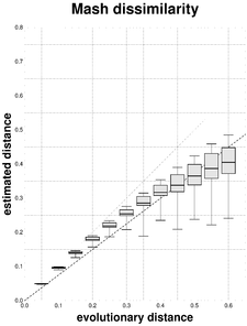
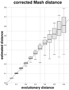
Box plots representing the mean, lower and upper quartiles, and 25th and 975th permilles of \(N\) = 500 estimates \(\hat{d}\) of the evolutionary distances \(d\) = 0.05, 0.10, ..., 0.60. Each linear regression through the origin with slope value b is represented with dashed lines.
b: Results obtained with the F81-corrected Mash distance; slope b = 1.0338, coefficient of determination of all points R2 = 0.9736, coefficient of determination of the 12 mean points R2 = 0.9998.
As expected (e.g.
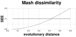
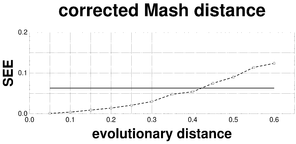
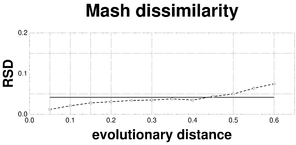
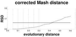
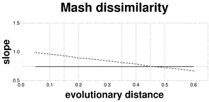
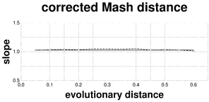
Plots associated to the data represented in Fig.
b: SEE plot of the F81-corrected Mash distance; reference SEE = 0.0638.
c: RSD plot of the Mash dissimilarity; reference RSD = 0.0426.
d: RSD plot of the F81-corrected Mash distance; reference RSD = 0.0626.
e: Linear slope plot of the Mash dissimilarity; reference slope = 0.7491.
f: Linear slope plot of the F81-corrected Mash distance; reference slope = 1.0338.
As JolyTree is expected to accurately estimate the evolutionary distance \(d\) between every pair of genomes that are not too distant (e.g. \(d\) < 0.5), this bioinformatics procedure is recommended for quickly inferring phylogenetic trees from genomes belonging to the same genus. It was used to reconstruct a phylogenetic tree from the \(n\) = 96 Listeria genome contig sets generated by
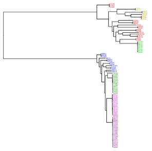
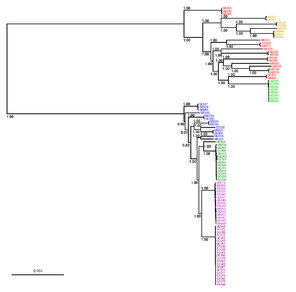
Model tree used for genome data simulation by
b: Inferred tree with branch support (rate of elementary quartets) represented only at each branch of length > 0.00005; scale bar refers to 0.004 nucleotide substitutions per character.
To measure the overall phylogenetic signal induced by the estimated distances, the Arboricity coefficient (arb;
Real-case analyses
To observe the ability of JolyTree to quickly infer accurate species trees from real data, genome assemblies from the RefSeq collection (
This representative collection of genome sequence sets shows that the GC content is very heterogeneous across genera (Suppl. material
It should be stressed that the data noising strategy had a moderate usefulness on these datasets, as no better tree (according to the BME criterion) than the one inferred by FastME alone was obtained for 125 datasets. This could be explained by the overall good treelikeness of the estimated evolutionary distances (Suppl. material
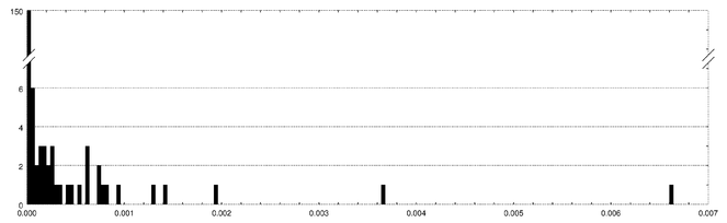
Distribution of the normalized Balanced Minimum Evolution (BME) tree length differences observed between phylogenetic trees inferred by FastME with and without the data noising strategy implemented by JolyTree. This distribution represents 187 observed values \(\Delta(T_0, T) = (\ell(T_0)-\ell(T))/\ell(T_0)\), where \(T_0\) is the tree inferred by FastME alone, \(T\) the one inferred by JolyTree via the data noising strategy, and \(\ell(T)\) the BME tree length estimate of \(T\). A tree \(T\) is considered as more accurate that \(T_0\) when \(\Delta(T_0, T)\) > 0.
Thanks to its ability to run on multiple threads, JolyTree is quite fast. On an Intel Xeon E5-1660 v4 (16Gb RAM) running under Linux Debian 4.9.110-3+deb9u6, 90% of the 187 genome datasets were analyzed in less than 15 and 5 minutes each, on 6 and 12 threads, respectively. The main variable having a negative impact on the overall running times is the number \( n\) of genomes, e.g. with quite comparable genome sizes (e.g. \(\overline{g}\) = 6.5 Mb), observed running times varied from 69 and 46 seconds with \(n\) = 30 (Duganella) to 30 and 19 minutes with \(n\) = 291 (Rhizobium) on 6 and 12 threads, respectively. Average genome size \(\overline{g}\) has less impact on the overall running times, as it only slows the Mash sketching step, e.g. with \(n\) = 34, observed running times varied from 62 and 16 seconds with \(\overline{g}\) = 2.8 Mb (Caldicellulosiruptor) to 4 and 3 minutes with \(\overline{g}\) = 34.1 Mb (Aspergillus) on 6 and 12 threads, respectively. JolyTree therefore represents a useful tool to quickly infer phylogenetic trees from large sets of genome sequences on standard computers.
Finally, to illustrate the accuracy of the phylogenetic trees inferred by JolyTree, a bibliographical survey was performed for each of the 187 genera to find recently published phylogenetic trees for comparison. Considering only genome datasets made up by at least four species, as well as only robust phylogenomics analyses based on core genome data for comparison, this survey led to six genera: Aggregatibacter (
The Aggregatibacter tree inferred by JolyTree (Fig.
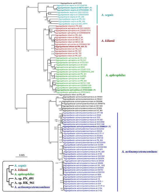
Phylogenetic tree inferred by JolyTree from the RefSeq genomes belonging to the genus Aggregatibacter. For each type strain (in bold), the clade determined by the isolates expected to belong to the same species (e.g. estimated pairwise distances < 0.05) is labeled by the species name and colored accordingly. Leaf names were automatically generated. Scale bar corresponds to an estimated evolutionary distance of 0.025. The inset summarizes a model tree of the Aggregatibacter species based on the phylogenetic analysis of
The Borreliella tree inferred by JolyTree is represented in Fig.
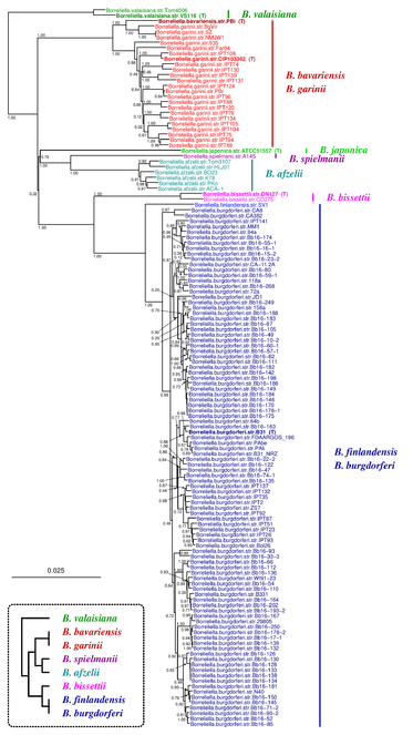
Phylogenetic tree inferred by JolyTree from the RefSeq genomes belonging to the genus Borreliella. For each type strain (in bold), the clade determined by the isolates expected to belong to the same species (e.g. estimated pairwise distances < 0.05) is labeled by the species name and colored accordingly. Leaf names were automatically generated. Scale bar corresponds to an estimated evolutionary distance of 0.025. The inset summarizes a model tree of the Borreliella species based on the phylogenetic analysis of
Concerning the genus Elizabethkingia, two recently published conflicting phylogenetic trees exist (inset in Fig.
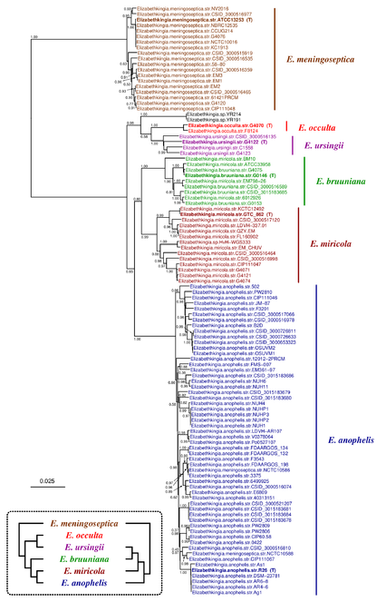
Phylogenetic tree inferred by JolyTree from the RefSeq genomes belonging to the genus Elizabethkingia. For each type strain (in bold), the clade determined by the isolates expected to belong to the same species (e.g. estimated pairwise distances < 0.05) is labeled by the species name and colored accordingly. Leaf names were automatically generated. Scale bar corresponds to an estimated evolutionary distance of 0.025. The inset summarizes two model trees of the Elizabethkingia species based on the phylogenetic analyses of
The Lactococcus tree inferred by JolyTree (Fig.
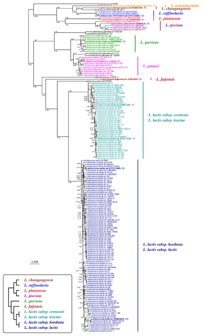
Phylogenetic tree inferred by JolyTree from the RefSeq genomes belonging to the genus Lactococcus. For each type strain (in bold), the clade determined by the isolates expected to belong to the same species (e.g. estimated pairwise distances < 0.05) is labeled by the species name and colored accordingly. Leaf names were automatically generated. Scale bar corresponds to an estimated evolutionary distance of 0.025. The inset summarizes a model tree of the Lactococcus species based on the phylogenetic analysis of
The Providencia tree inferred by JolyTree is represented in Fig.
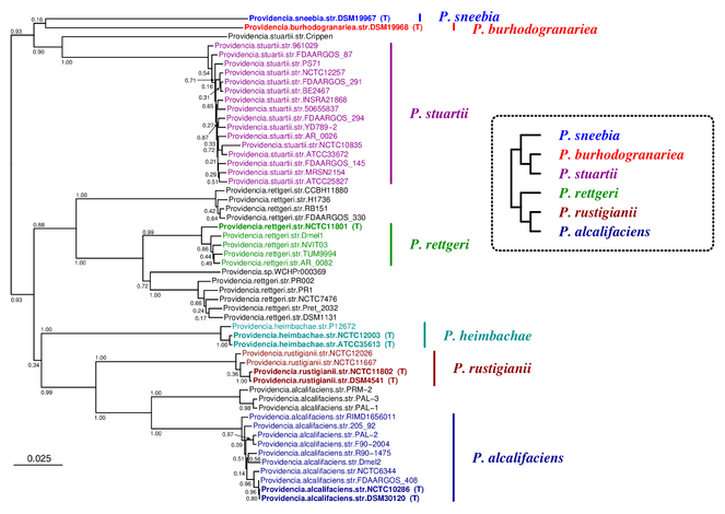
Phylogenetic tree inferred by JolyTree from the RefSeq genomes belonging to the genus Providencia. For each type strain (in bold), the clade determined by the isolates expected to belong to the same species (e.g. estimated pairwise distances < 0.05) is labeled by the species name and colored accordingly. Leaf names were automatically generated. Scale bar corresponds to an estimated evolutionary distance of 0.025. The inset summarizes a model tree of the Providencia species based on the phylogenetic analysis of
The phylogenetic relationships among Ralstonia species was deeply studied by
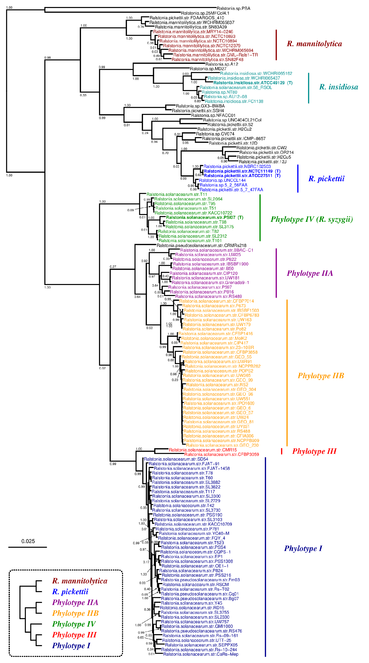
Phylogenetic tree inferred by JolyTree from the RefSeq genomes belonging to the genus Ralstonia. For each type strain (in bold), the clade determined by the isolates expected to belong to the same species (e.g. estimated pairwise distances < 0.05) is labeled by the species name and colored accordingly. Leaf names were automatically generated. Scale bar corresponds to an estimated evolutionary distance of 0.025. The inset summarizes a model tree of the Ralstonia species based on the phylogenetic analysis of
These detailed phylogenetic analyses of the six genera Aggregatibacter, Borreliella, Elizabethkingia, Lactococcus, Providencia and Ralstonia show that JolyTree is a useful tool to quickly infer species trees from whole genome assemblies that are comparable with trees reconstructed from the concatenation of large sets of multiple homologous sequence alignments. They also show that these phylogenetic trees are practical representations to detect new species within a bacterial genus.
Conclusions
This paper describes a novel bioinformatics procedure, implemented by the Bash script JolyTree (gitlab.pasteur.fr/GIPhy/JolyTree), to perform a complete phylogenetic analysis from unaligned genome sequence sets. Such procedure is quite fast because it takes advantage of the ability of the pairwise distance estimate step to be run on multiple threads. Simulation and real case analyses have shown that JolyTree leads to accurate trees. Some incorrect branching can be observed within the inferred phylogenetic trees, but they are often assessed by weak branch supports. Therefore, JolyTree represents a useful approach for performing phylogenetic analyses with fast running times from hundreds of genome assemblies. Of note, this bioinformatics procedure was used previously for inferring Corynebacterium (
More generally, this paper confirms the usefulness of the MinHash dissimilarity and its ability to efficiently approximate the pairwise p-distance (and the related ANI similarity) between two genome contig sets. However, this paper highlights the importance of transforming a p-distance value into an evolutionary distance estimate in the context of phylogenetic inference, especially when p-distance values are large (e.g. > 0.1). The use of the F81-transformation represents a very simple but efficient way to quickly obtain efficient pairwise evolutionary distance estimates. Of note, such transformation can be easily adaptated with future implementations of the pairwise Mash dissimilarities (e.g.
Acknowledgements
This manuscript is dedicated to the memory of Nicolas Joly, who helped to improve the implementation of the script JolyTree for running on multiple threads. The author thanks Laetitia Fabre, Julien Guglielmini and Rachel Legendre for useful comments on the manuscript. The author is also grateful to Brian D. Ondov for reviewing this manuscript. The author is obliged to Sylvain Brisse and to the Hub de Bioinformatique et Biostatistique, Institut Pasteur, Paris (France), for support.
Author contributions
AC conceived the presented idea, implemented the script, conceived the simulations, performed the computations, and wrote the manuscript.
Conflicts of interest
No conflict of interest to declare.
References
-
Genome BLAST distance phylogenies inferred from whole plastid and whole mitochondrion genome sequences.BMC Bioinformatics7(1):350. https://doi.org/10.1186/1471-2105-7-350
-
Dashing: fast and accurate genomic distances with HyperLogLog.bioRxivhttps://doi.org/10.1101/501726
-
Weighted Neighbor Joining: a likelihood-based approach to distance-based phylogeny reconstruction.Molecular Biology and Evolution17(1):189‑197. https://doi.org/10.1093/oxfordjournals.molbev.a026231
-
The recovery of trees from measures of dissimilarity. In: Hodson FR, Kendall DG, Tautu P (Eds)Mathematics in Archaeological and Historical Sciences.Edinburgh University Press,Edimburgh,387-395pp. URL: http://homepages.inf.ed.ac.uk/opb/homepagefiles/phylogeny-scans/manuscripts.pdf
-
Primordial origin and diversification of plasmids in Lyme disease agent bacteria.BMC Genomics19(1). https://doi.org/10.1186/s12864-018-4597-x
-
Next-generation phylogenomics.Biology Direct8(1). https://doi.org/10.1186/1745-6150-8-3
-
Inferring phylogenies of evolving sequences without multiple sequence alignment.Scientific Reports4(1). https://doi.org/10.1038/srep06504
-
Exploration of phylogenetic data using a global sequence analysis method.BMC Evolutionary Biology5(1):63. https://doi.org/10.1186/1471-2148-5-63
-
The noising method: a new method for combinatorial optimization.Operations Research Letters14(3):133‑137. https://doi.org/10.1016/0167-6377(93)90023-A
-
Detecting phylogenetic signals in eukaryotic whole genome sequences.Journal of Computational Biology19(8):945‑56. https://doi.org/10.1089/cmb.2012.0122
-
Barcoding's next top model: an evaluation of nucleotide substitution models for specimen identification.Methods in Ecology and Evolution3(3):457‑465. https://doi.org/10.1111/j.2041-210x.2011.00176.x
-
Bioinformatic genome comparisons for taxonomic and phylogenetic assignments using Aeromonas as a test case.mBio5(6). https://doi.org/10.1128/mbio.02136-14
-
SDM: a fast distance-based approach for (super)tree building in phylogenomics.Systematic Biology55(5):740‑755. https://doi.org/10.1080/10635150600969872
-
morePhyML: Improving the phylogenetic tree space exploration with PhyML 3.Molecular Phylogenetics and Evolution61(3):944‑948. https://doi.org/10.1016/j.ympev.2011.08.029
-
Taxonomic status of Corynebacterium diphtheriae biovar Belfanti and proposal of Corynebacterium belfantii sp. nov.International Journal of Systematic and Evolutionary Microbiology68(12):3826‑3831. https://doi.org/10.1099/ijsem.0.003069
-
The consistency of several phylogeny-inference methods under varying evolutionary rates.Molecular Biology and Evolution9(3):537‑551. https://doi.org/10.1093/oxfordjournals.molbev.a040740
-
A genomic distance based on MUM indicates discontinuity between most bacterial species and genera.Journal of Bacteriology191(1):91‑99. https://doi.org/10.1128/jb.01202-08
-
A novel method of characterizing genetic sequences: genome space with biological distance and applications.PloS one6(3):e17293. https://doi.org/10.1371/journal.pone.0017293
-
PTreeRec: phylogenetic tree reconstruction based on genome BLAST distance.Computational Biology and Chemistry30(4):300‑302. https://doi.org/10.1016/j.compbiolchem.2006.04.003
-
Fast and accurate phylogeny reconstruction algorithms based on the minimum-evolution principle.Journal of Computational Biology9(5):687‑705. https://doi.org/10.1089/106652702761034136
-
Theoretical foundation of the Balanced Minimum Evolution method of phylogenetic inference and its relationship to weighted least-squares tree fitting.Molecular Biology and Evolution21(3):587‑598. https://doi.org/10.1093/molbev/msh049
-
Efficient estimation of pairwise distances between genomes.Bioinformatics (Oxford, England)25(24):3221‑7. https://doi.org/10.1093/bioinformatics/btp590
-
Evolutionary trees from DNA sequences: A maximum likelihood approach.Journal of Molecular Evolution17(6):368‑376. https://doi.org/10.1007/bf01734359
-
How independent are the appearances of n-mers in different genomes?Bioinformatics20(15):2421‑2428. https://doi.org/10.1093/bioinformatics/bth266
-
Comparative genomics of bacteria in the genus Providencia isolated from wild Drosophila melanogaster.BMC Genomics13(1):612. https://doi.org/10.1186/1471-2164-13-612
-
Genome-based phylogeny of dsDNA viruses by a novel alignment-free method.Gene492(1):309‑14. https://doi.org/10.1016/j.gene.2011.11.004
-
Outbreak of invasive wound Mucormycosis in a burn unit due to multiple strains of Mucor circinelloides f. circinelloides resolved by whole-genome sequencing.mBio9(2):e00573‑18. https://doi.org/10.1128/mBio.00573-18
-
Neighbor-Joining revealed.Molecular Biology and Evolution23(11):1997‑2000. https://doi.org/10.1093/molbev/msl072
-
DNA–DNA hybridization values and their relationship to whole-genome sequence similarities.International Journal of Systematic and Evolutionary Microbiology57(1):81‑91. https://doi.org/10.1099/ijs.0.64483-0
-
Can we have confidence in a tree representation?In: Gascuel O, Sagot MF (Eds)Computational Biology, LNCS.Springer Berlin Heidelberg,Berlin, Heidelberg,45-56pp. https://doi.org/10.1007/3-540-45727-5_5
-
A phylogenetic analysis of the brassicales clade based on an alignment-free sequence comparison method.Frontiers in plant science3:192. https://doi.org/10.3389/fpls.2012.00192
-
Estimating mutation distances from unaligned genomes.Journal of Computational Biology16(10):1487‑500. https://doi.org/10.1089/cmb.2009.0106
-
andi: Fast and accurate estimation of evolutionary distances between closely related genomes.Bioinformatics31(8):1169‑1175. https://doi.org/10.1093/bioinformatics/btu815
-
Whole-genome prokaryotic phylogeny.Bioinformatics21(10):2329‑2335. https://doi.org/10.1093/bioinformatics/bth324
-
Application and accuracy of molecular phylogenies.Science264(5159):671‑677. https://doi.org/10.1126/science.8171318
-
δ Plots: A tool for analyzing phylogenetic distance data.Molecular Biology and Evolution19(12):2051‑2059. https://doi.org/10.1093/oxfordjournals.molbev.a004030
-
Spaced words and kmacs: fast alignment-free sequence comparison based on inexact word matches.Nucleic Acids Research42(Web Server issue):7‑11. https://doi.org/10.1093/nar/gku398
-
Alignment-free comparison of genome sequences by a new numerical characterization.Journal of Theoretical Biology281(1):107‑12. https://doi.org/10.1016/j.jtbi.2011.04.003
-
Performance of phylogenetic methods in simulation.Systematic Biology44(1):17‑48. https://doi.org/10.1093/sysbio/44.1.17
-
Limitations of the evolutionary parsimony method of phylogenetic analysis.Molecular Biology and Evolution7(1):82‑102. https://doi.org/10.1093/oxfordjournals.molbev.a040588
-
Evolution of protein molecules. In: Munro HN (Ed.)Mammalian protein metabolism.III.Academic Press,New York,21-132pp. https://doi.org/10.1016/B978-1-4832-3211-9.50009-7
-
On the stochastic model for estimation of mutational distance between homologous proteins.Journal of Molecular Evolution2(1):87‑90. https://doi.org/10.1007/bf01653945
-
Alignment-free distance measure based on return time distribution for sequence analysis: applications to clustering, molecular phylogeny and subtyping.Molecular Phylogenetics and Evolution65(2):510‑22. https://doi.org/10.1016/j.ympev.2012.07.003
-
Benzalkonium tolerance genes and outcome in Listeria monocytogenes meningitis.Clinical Microbiology and Infection23(4):1‑265. https://doi.org/10.1016/j.cmi.2016.12.008
-
Insights from 20 years of bacterial genome sequencing.Functional & Integrative Genomics15(2):141‑161. https://doi.org/10.1007/s10142-015-0433-4
-
Evaluation of phylogenetic reconstruction methods using bacterial whole genomes: a simulation based study.Wellcome Open Research3:33. https://doi.org/10.12688/wellcomeopenres.14265.2
-
FastME 2.0: A comprehensive, accurate, and fast distance-based phylogeny inference program.Molecular Biology and Evolution32(10):2798‑2800. https://doi.org/10.1093/molbev/msv150
-
Fast alignment-free sequence comparison using spaced-word frequencies.Bioinformatics30(14):1991‑9. https://doi.org/10.1093/bioinformatics/btu177
-
Fast and accurate phylogeny reconstruction using filtered spaced-word matches.Bioinformatics33(7):971‑979. https://doi.org/10.1093/bioinformatics/btw776
-
Coronavirus phylogeny based on base-base correlation.International Journal of Bioinformatics Research and Applications4(2):211‑20. https://doi.org/10.1504/IJBRA.2008.018347
-
A novel fast vector method for genetic sequence comparison.Scientific Reports7(1). https://doi.org/10.1038/s41598-017-12493-2
-
Twisted trees and inconsistency of tree estimation when gaps are treated as missing data – The impact of model mis-specification in distance corrections.Molecular Phylogenetics and Evolution93:289‑295. https://doi.org/10.1016/j.ympev.2015.07.027
-
Highly parallelized inference of large genome-based phylogenies.Concurrency and Computation: Practice and Experience26(10):1715‑1729. https://doi.org/10.1002/cpe.3112
-
Increasing the efficiency of searches for the Maximum Likelihood tree in a phylogenetic analysis of up to 150 nucleotide sequences.Systematic Biology56(6):988‑1010. https://doi.org/10.1080/10635150701779808
-
Whole-genome sequencing of Aggregatibacter species isolated from human clinical specimens and description of Aggregatibacter kilianii sp. nov.Journal of Clinical Microbiology56(7). https://doi.org/10.1128/jcm.00053-18
-
Meat and fish as sources of extended-spectrum β-lactamase–producing Escherichia coli, Cambodia.Emerging Infectious Diseases25(1). https://doi.org/10.3201/eid2501.180534
-
Evolutionary change in DNA sequences. In: Nei M, Kumar S (Eds)Molecular Evolution and Phylogenetics.Oxford University Press,New York,33-50pp. URL: https://global.oup.com/academic/product/molecular-evolution-and-phylogenetics-9780195135855 [ISBN9780195135855].
-
Revisiting the taxonomy of the genus Elizabethkingia using whole-genome sequencing, optical mapping, and MALDI-TOF, along with proposal of three novel Elizabethkingia species: Elizabethkingia bruuniana sp. nov., Elizabethkingia ursingii sp. nov., and Elizabethkingia occulta sp. nov.Antonie van Leeuwenhoek111(1):55‑72. https://doi.org/10.1007/s10482-017-0926-3
-
Reference sequence (RefSeq) database at NCBI: current status, taxonomic expansion, and functional annotation.Nucleic Acids Research44(D1):D733‑D745. https://doi.org/10.1093/nar/gkv1189
-
Mash: fast genome and metagenome distance estimation using MinHash.Genome Biology17(1). https://doi.org/10.1186/s13059-016-0997-x
-
Distance-based methods in phylogenetics. In: Kliman R (Ed.)Encyclopedia of Evolutionary Biology.1st Edition.Academic Press,458-465pp. URL: https://hal-lirmm.ccsd.cnrs.fr/lirmm-01386569 [ISBN9780128000496].
-
Direct calculation of a tree length using a distance matrix.Journal of Molecular Evolution51(1):41‑47. https://doi.org/10.1007/s002390010065
-
Evolutionary dynamics and genomic features of the Elizabethkingia anophelis 2015 to 2016 Wisconsin outbreak strain.Nature Communications8:15483. https://doi.org/10.1038/ncomms15483
-
Evolutionary implications of microbial genome tetranucleotide frequency biases.Genome Research13(2):145‑158. https://doi.org/10.1101/gr.335003
-
Seq-Gen: an application for the Monte Carlo simulation of DNA sequence evolution along phylogenetic trees.Computer applications in the biosciences : CABIOS13(3):235‑8.
-
Genome-scale approaches to resolving incongruence in molecular phylogenies.Nature425(6960):798‑804. https://doi.org/10.1038/nature02053
-
When is it safe to use an oversimplified substitution model in tree-making?Molecular Biology and Evolution13(9):1255‑1265. https://doi.org/10.1093/oxfordjournals.molbev.a025691
-
The neighbor-joining method: a new method for reconstructing phylogenetic trees.Molecular Biology and Evolution4(4):406‑425. https://doi.org/10.1093/oxfordjournals.molbev.a040454
-
Relative efficiencies of the Fitch-Margoliash, Maximum-Parsimony, Maximum-Likelihood, Minimum-Evolution, and Neighbor-Joining methods of phylogenetic tree construction in obtaining the correct tree.Molecular Biology and Evolution6(5):514‑525. https://doi.org/10.1093/oxfordjournals.molbev.a040572
-
Alignment-free genome comparison with feature frequency profiles (FFP) and optimal resolutions.Proceedings of the National Academy of Sciences of the United States of America106(8):2677‑2682. https://doi.org/10.1073/pnas.0813249106
-
Whole-genome phylogeny of Escherichia coli/Shigella group by feature frequency profiles (FFPs).Proceedings of the National Academy of Sciences of the United States of America108(20):8329‑8334. https://doi.org/10.1073/pnas.1105168108
-
A statistical method for evaluating systematic relationships.University of Kansas Science Bulletin38:1409‑1438. URL: https://ia800707.us.archive.org/33/items/cbarchive_33927_astatisticalmethodforevaluatin1902/astatisticalmethodforevaluatin1902.pdf
-
A note on the neighbor-joining algorithm of Saitou and Nei.Molecular Biology and Evolution5(6):729‑731. https://doi.org/10.1093/oxfordjournals.molbev.a040527
-
On Inconsistency of the Neighbor-Joining, Least Squares, and Minimum Evolution estimation when substitution processes are incorrectly modeled.Molecular Biology and Evolution21(9):1629‑1642. https://doi.org/10.1093/molbev/msh159
-
Biases of the estimates of DNA divergence obtained by the restriction enzyme technique.Journal of Molecular Evolution18(2):115‑120. https://doi.org/10.1007/bf01810830
-
Estimation of evolutionary distance between nucleotide sequences.Molecular Biology and Evolution1(3):269‑285. https://doi.org/10.1093/oxfordjournals.molbev.a040317
-
Evolutionary distance estimation under heterogeneous substitution pattern among lineages.Molecular Biology and Evolution19(10):1727‑1736. https://doi.org/10.1093/oxfordjournals.molbev.a003995
-
BMScan: using whole genome similarity to rapidly and accurately identify bacterial meningitis causing species.BMC Infectious Diseases18(1). https://doi.org/10.1186/s12879-018-3324-1
-
The Harvest suite for rapid core-genome alignment and visualization of thousands of intraspecific microbial genomes.Genome Biology15(11). https://doi.org/10.1186/s13059-014-0524-x
-
The average common substring approach to phylogenomic reconstruction.Journal of Computational Biology13(2):336‑50. https://doi.org/10.1089/cmb.2006.13.336
-
The spectrum of genomic signatures: from dinucleotides to chaos game representation.Gene346:173‑85. https://doi.org/10.1016/j.gene.2004.10.021
-
CVTree update: a newly designed phylogenetic study platform using composition vectors and whole genomes.Nucleic Acids Research37:W174‑W178. https://doi.org/10.1093/nar/gkp278
-
Large local analysis of the unaligned genome and its application.Journal of Computational Biology20(1):19‑29. https://doi.org/10.1089/cmb.2011.0052
-
Maximum-likelihood estimation of phylogeny from DNA sequences when substitution rates differ over sites.Molecular Biology and Evolutionhttps://doi.org/10.1093/oxfordjournals.molbev.a040082
-
Estimating the pattern of nucleotide substitution.Journal of Molecular Evolution39(1):105‑11.
-
Co-phylog: an assembly-free phylogenomic approach for closely related organisms.Nucleic Acids Research41(7):e75. https://doi.org/10.1093/nar/gkt003
-
Phylogenetic analysis reveals the taxonomically diverse distribution of the Pseudomonas putida group.The Journal of General and Applied Microbiology63(1):1‑10. https://doi.org/10.2323/jgam.2016.06.003
-
A novel construction of genome space with biological geometry.DNA Research17(3):155‑68. https://doi.org/10.1093/dnares/dsq008
-
Genome-level comparisons provide insight into the phylogeny and metabolic diversity of species within the genus Lactococcus.BMC Microbiology17:213. https://doi.org/10.1186/s12866-017-1120-5
-
Proper distance metrics for phylogenetic analysis using complete genomes without sequence alignment.International Journal of Molecular Sciences11(3):1141‑1154. https://doi.org/10.3390/ijms11031141
-
ПОСТРОЕНИЕ ДЕРЕВА ПО НАБОРУ РАССТОЯНИЙ МЕЖДУ ВИСЯЧИМИ ВЕРШИНАМИ.Uspekhi Matematicheskikh Nauk20(6):90‑92. [InRussian]. URL: http://mi.mathnet.ru/eng/umn6134
-
Phylogenomic analysis of the genus Ralstonia based on 686 single-copy genes.Antonie van Leeuwenhoek109(1):71‑82. https://doi.org/10.1007/s10482-015-0610-4
-
BinDash, software for fast genome distance estimation on a typical personal laptop.Bioinformaticshttps://doi.org/10.1093/bioinformatics/bty651
-
Alignment-free sequence comparison: benefits, applications, and tools.Genome Biology18(1). https://doi.org/10.1186/s13059-017-1319-7
Supplementary materials
For each genus, the table reports the number of genomes (no. taxa), the mean genome sequence size (mean genome size) and the associated standard deviation (SD genome size), the mean percentage of observed GC content (mean %GC) and the associated standard deviation (SD %GC), the largest estimated Mash dissimilarity (max Mash dissimilarity) and F81-corrected Mash distance (max F81 distance), the treelikeness coefficients (arboricity and mean delta), the proportion of external negative branches (% negative branch), the mean rate of elementary quartets (mean branch support) and the associated standard deviation (SD branch support), and the inferred phylogenetic tree in NEWICK format.
Download file (351.50 kb)
Each raw contains the taxon name used during the JolyTree analysis (column 1), followed by the corresponding entry from the RefSeq assembly report (ftp.ncbi.nlm.nih.gov/genomes/ASSEMBLY_REPORTS/assembly_summary_refseq.txt).
Download file (764.46 kb)