|
Research Ideas and Outcomes :
Review Article
|
|
Corresponding author: Alex Hardisty (hardistyar@cardiff.ac.uk), Laurence Livermore (l.livermore@nhm.ac.uk)
Received: 23 Sep 2020 | Published: 29 Sep 2020
© 2020 Alex Hardisty, Laurence Livermore, Stephanie Walton, Matt Woodburn, Helen Hardy
This is an open access article distributed under the terms of the Creative Commons Attribution License (CC BY 4.0), which permits unrestricted use, distribution, and reproduction in any medium, provided the original author and source are credited.
Citation:
Hardisty A, Livermore L, Walton S, Woodburn M, Hardy H (2020) Costbook of the digitisation infrastructure of DiSSCo. Research Ideas and Outcomes 6: e58915. https://doi.org/10.3897/rio.6.e58915
|
|
Abstract
There has been little work to compare and understand the operating costs of digitisation using a standardised approach. This paper discusses a first attempt at gathering digitisation cost information from multiple institutions and analysing the data. This paper has been written: for other digitisation managers who want to breakdown and compare project costs; as a potential baseline for future digitisation projects; as a starting point for prioritising research and development to reduce digitisation costs.
Keywords
natural history collections, operational costs, cost analysis, specimen digitisation
Executive summary
This report focuses on analysing the operating costs of digitisation and developing a standardised method for gathering cost information from partners within the Distributed System of Scientific Collections Project (DiSSCo https://www.dissco.eu) as part of the Innovation and consolidation for large scale digitisation of natural heritage project (ICEDIG https://icedig.eu). Data was collected from seven institutions: Botanic Garden Meise (APM), Royal Botanic Garden Kew (RBGK), Royal Belgian Institute of Natural Sciences (RBINS), Finnish Museum of Natural History (LUOMUS), National Museum of Natural History France (MNHN), Natural History Museum and Botanical Garden Tartu (UTARTU) and Natural History Museum London (NHMUK). Between them they contributed a total of 35 costbooks on different collection types and categories. While institutions varied in how they categorized and reported their costs, the costbook format provided a consistent and reliable template from which to compare costs between institutions and collection types, to assess how costs are related to the pace of digitisation (throughput) and where the greatest costs – and cost differences – can be found.
Each institution was asked to break down their digitisation costs into three categories: capital costs (equipment, cameras, workstations, etc.), fixed costs (space charges, depreciation, fixed-cost staff) and variable costs (labour costs based on time and throughput, consumables). Institutions were also asked to report on the number of staff, their throughput (the number of specimens digitised per month) and the time spent digitising a specimen. Costbooks were grouped according to the type of collection, which included herbarium, fungarium, palaeontological, spirit material, etc. However, some collections, such as vertebrates, only had one reported case while six costbooks were returned for herbarium collections. Thus costings are reliable for some collection types while other collections types will require further research and confirmation.
Digitisation costs varied according to several different factors. The most dramatic difference was between the cost of digitising different types of collections. Vertebrates and marine invertebrates were shown to be significantly more costly to digitise than herbarium and pinned insects. This may be due to differences in speed and efficiency gains that can be achieved with 2D or flat objects versus 3D objects, but is also indicative of the higher priority given to these collections types and the subsequent improved workflows that have developed over time compared to those collections that are being digitised in smaller numbers.
Cost variances were also reported within the same collection types. Multiple cases were returned for herbarium, pinned insects, microscope slides, paleontogical and fungarium collections but with wide variances in cost in some cases. One institution reported €3.89 PPS (Purchasing Power Standard) per paleontology item versus another that reported €28.28 PPS. Further data collection for collections types with a wide cost range may result in more normalised data. While the range was not quite as wide for collections that had a larger sample size, some institutions still reported double the cost per item than others.
The major contributor to these cost differences was staffing and labour which proved to be the largest cost component in all cases. However, no distinct correlation was found between the number of staff and the total annual throughput of specimens. An increase in staff numbers did not predict an increase in throughput. The throughput for a staff of one for herbarium and pinned insect collections ranged from approximately 20,000 to 130,000 specimens per year, indicating that the greatest efficiency gains are achieved through improvements to workflow rather than an increase in staff. However, more research is required on why such a wide range in throughput was reported and the specific differences in equipment and workflow that contributed to it.
Considering the complexities of the digitisation process, and its variability among institutions and between different types of collections, we conclude that time spent (and the associated labour costs) is an essential variable that informs cost. While this report should not be considered a forecasting tool for predicting anticipated costs, it does offer insight into which costs should be accounted for and where attention should be focussed to increase throughput and reduce costs.
1. Introduction
This is the first attempt to gather and analyse the costs of constructing and operating the digitisation infrastructure of the DiSSCo project as a distributed infrastructure for digitisation. This deliverable report focuses on the operating costs of digitisation and standardising the gathering of cost information from DiSSCo partners.
In this report, we have incorporated the costbook methodology along with the completed institutional costbooks from the collection holding institutes within the ICEDIG Project. We have made a preliminary analysis of the completed costbooks that leads to some observations and recommendations. By harmonising approaches to gather costbook information and reporting gathered costs in terms of the European Union-wide ‘Purchasing Power Standard’ (PPS), we aim to take account of the different purchasing power of money in different Member State economies, and to represent costs normalised for the EU as a whole. We believe this is a pragmatic approach to cost reporting that can also be used for DiSSCo budgeting.
1.1 Project context
This project report was written as a formal Deliverable (D8.2) of the ICEDIG Project and was previously made available to project partners and submitted to the European Commision as a report. While the differences between these versions are minor the authors consider this the definitive version of the report.
The following text is the formal task description (Task 8.4) from the ICEDIG project's Description of the Action (workplan):
This task will gather the complete costs of constructing and operating DiSSCo as a distributed infrastructure for digitisation. The costs of different methods of digitisation must be identified (i.e. per design alternatives described by task 8.3) and entered in a ‘ Costbook ’ (D8.2). The costs of constructing the infrastructure must be itemised. A basic principle is that the full costs of all construction and operations activities must be itemised, irrespective of any expectation that these elements are already available or could be offered for free (or with a reduced price or as in-kind contribution). Output: ‘ Costbook ’, itemising costs of construction and operation of the infrastructure (D8.2). Services as input material to design the business model (task 8.5).
1.2 Constraining the scope of the task
A variation (narrowing) of the scope of the task description was agreed with the project Coordinator (January 2019), focusing only on the costs of approaches to mass digitisation as practised across multiple museums and avoiding unnecessary overlaps with the work to be done in the DiSSCo Prepare project. This aligns with the objectives of ICEDIG to concentrate on looking at innovations/efficiencies of digitisation, whilst the broader costs of building/operating DiSSCo are better dealt with in the DiSSCo Prepare project; where there is a whole work package (WP4) on financial readiness, including costing of construction and operation. The present task must contribute what DiSSCo Prepare needs for its work on achieving financial readiness.
2. Methodology for costing
2.1 Components of costs
Following basic cost accounting principles, we identify several components of costs:
Capital costs: Capital costs are fixed, one-time costs incurred on the purchase of equipment, buildings, construction to be used for digitisation. In other words, it is the total cost of bringing a digitisation facility to operational readiness. If in doubt about what to count as capital, a general rule is that if an asset has a useful life of more than one year, it is a capital cost.
While outright purchase of equipment and space is most common, it is sometimes possible to lease assets for a period. The terms of any lease – in particular, whether there is an option to acquire the asset e.g., at the end of the lease – affect whether the cost is treated as capital or as an operating cost.
Operating costs: Sometimes known as running costs or revenue costs; operating costs are the ongoing expenses related to carrying out business, in this case digitisation. Operating costs can be fixed or variable. Fixed costs are unrelated to the volume of specimens digitised. No matter how high or low are the rates of digitisation, fixed costs remain the same. Variable costs, on the other hand, show a relationship (normally linear) between the volume of specimens digitised and total variable costs.
Fixed operating costs: Fixed operating costs are expenses incurred for operating a digitisation facility that are not dependent on the level of usage. These costs are incurred for as long as a facility is operational (but not necessarily operating). No matter how high or low are the rates of digitisation, costs remain the same. Fixed costs can be non-recurring (one-off) expenses, such as replacement parts, or recurring expenses, such as monthly maintenance contract, salaries, building/floor rental, heating and lighting, etc. Sometimes, fixed costs are split into direct fixed costs i.e., those costs that can be easily and directly associated with the facility itself, and indirect or overhead costs (normally, costs of space, electricity, heating, lighting, general administrative staff, etc.) that are incurred by an institution as a whole but which cannot be directly attributed to specific activities, Indirect or overhead costs are normally apportioned on a percentage basis to different departments, facilities, etc.
Variable operating costs: Variable costs are recurring expenses incurred only when digitisation is taking place. They include rated labour costs (i.e., per hour costs of staff carrying out digitisation tasks, who don’t work, or who work on other tasks, when digitisation is not taking place) and consumable materials used during the digitisation process, such as barcode labels. The amount of these costs depends upon the scale of the digitisation activity. The level and type of digitisation affects variable costs. Costs may depend on the amount of data to be recorded, the difficulty of working with that data (e.g., in transcription), and the number of images to be made. Recording just the unique code and taxon name of a specimen takes less time than recording all information available for a specimen. Some specimen categories take longer to process than others.
2.2 Marginal costs
It can be helpful to consider the marginal costs associated with digitising one additional specimen (or collection). Understanding these costs can be helpful for comparisons between approaches digitising single or small numbers of specimens, mass digitisation and digitisation-on-demand.
When an additional specimen can be digitised for less than the average cost of all previous digitisations of specimens, economies of scale are being achieved. The aim of introducing automation, for example is to force the marginal cost below the long-run average cost, so that the latter eventually falls. Conversely, there may be approaches to digitisation – for example dealing with special requests - where marginal cost is higher than average cost. In this case, a consequence of handling increasing numbers of special requests is potentially higher average costs overall.
2.3 Separating costs of digitisation
Costs of digitisation divide naturally into: i) establishment costs, meaning the upfront costs of building and equipping a digitisation facility, ii) costs of digitising specimens, and iii) costs of preserving that digitised data and making it findable, accessible, interoperable and re-usable (i.e., ‘FAIR’). A cost model identifying the main cost elements within each of (i) – (iii) (explained below) helps us to understand where the significant costs lie.
Nevertheless, different scenarios of digitisation, largely determined on whether digitisation is carried out in-house or outsourced, and at small versus large scale lead to different costs.*
Currently, most known digitisation initiatives fall into the in-house category, incurring capital costs for establishment and operating costs for running the facility. Some digitisation projects are undertaken on an outsourced/contract basis where a per item or total negotiated price is paid to cover the variable costs of digitisation, recoupment of contractor’s capital and fixed costs and provide a profit margin.
For the purposes of the present task we are mainly interested in the costs of establishing and operating in-house facilities but where possible to collect, it is also interesting to gather costs of outsourcing.
2.3.1 Cost of establishing a digitisation facility
Establishing a digitisation facility largely consists of capital costs, although it can also include other associated costs. Establishing a facility may often be treated as a capital project with a definite beginning and end and can include planning and specifying what is needed, tendering and procurement of equipment and/or services, readying the physical space where the facility is to be located, installation and testing of equipment, and finally, acceptance of the facility. If the intended facility is small, it may be treated as a small non-capital project e.g., the purchase of a single computer and camera as a digitisation workstation. A digitisation facility can be semi-permanent i.e., needed for a substantial time (e.g., several years) as part of a large digitisation programme; or it can be temporary for a specific digitisation project, such as when a specialist company contracts to digitise a specific collection(s) over a short period (e.g., weeks or months).
In many instances, capital and other establishment costs can support more than one digitisation workflow or operation. For instance, a computer, scanner or camera can be used with a variety of different collections. Reaching costs per workflow or per item therefore requires an apportionment by (approximate or actual) time spent using the equipment in different workflows. Any reasonable apportionment that avoids double counting of costs or excessive loading of capital costs in a way that distorts per item costs in a single workflow should be acceptable.
2.3.2 Cost of digitising specimens
The costs of digitising specimens and collections are operating costs. They must be considered as the result of a sequence of continuous or repetitive operations in a digitisation process that is performed to obtain digital object representations (i.e. digital specimens, labels, and/or collections of specimens like whole drawers, vials or palaeontological slabs) from physical objects, and the metadata that describes the digitisation process. We consider a digital object representation to potentially include transcribed data, analytical data (e.g., chemical, molecular) and data linked from other sources like literature. Cost units, which include components of both fixed costs (including depreciation of capital assets) and variable costs, must be averaged over the number of digital objects produced during the period needed to digitise.
It is clear there cannot be a single, common cost for digitisation. The fundamental differences of approach between digitisation-on-demand, project-driven digitisation and mass digitisation lead to quite different cost models. For a sense of this, just consider the different ways that just-in-time supply chains, cottage industries and automated factories operate. Costs can also vary depending on the level of digitisation desired (i.e., the sophistication: a bare level, a basic level, a regular level, or an extended level digitisation – as suggested by the proposed standard for Minimum Information about a Digital Specimen (MIDS)*
Digitisation occurs in different forms – by single specimen, by sub-part of a collection (e.g., tray of insects) – requiring different handling procedures and different digitisation approaches, according to the type of specimen. Herbarium sheets, which are almost two-dimensional and stored as sheets in folders and boxes are easily amenable to a high-speed approach involving a flat-bed conveyor and overhead camera. Pinned insects, on the other hand require more time-consuming mounting procedures and camera shots from multiple angles that are not just overhead. Spirit jars may need to be opened and emptied into a transparent tray and photographed from below, as well as above before being re-filled and sealed again. Retrieving a specimen from its storage, preparing/mounting it for digitisation, moving it through the process, repacking/preserving, and replacing it in cabinet/storage accounts (i.e., physically accessing and handling the specimen) accounts for almost all the cost of digitisation. Making the image(s) and databasing label information, even with the associated procedures of image processing, transcription and quality control is often not a substantial time-consuming element of the process and thus, not the largest part of the cost. Sometimes, opportunity is taken during digitisation to perform new conservation/preservation measures, such as re-mounting and re-labelling herbarium specimens. Such additional costs can complicate the picture, especially when the procedures are not applied for every specimen.
Digitisation processes can be separated into many discrete tasks performed. This has been shown by the analysis work of
Our five main activities of digitisation for cost gathering purposes are:
- Pre- and post- digitisation curation involves all tasks associated with retrieving specimens from storage; attaching and assigning barcodes; unpacking and preparing the specimen for digitisation, including essential conservation work; creating a CMS record if one does not already exist, and (if necessary) identification.
-
Specimen image capture includes setting up the imaging station; presenting specimens for imaging (e.g., positioning, via conveyor, etc.); making image(s); repacking and returning to storage after digitisation (can occur as part of (4)).
-
Image processing involves all tasks performed on an image or group of images after image acquisition, including: quality checks, control of image quality; barcode capture, file conversion, image cropping and colour/balance adjustments, other adjustments, segmentation, optical character recognition (OCR), etc.
-
Data capture is covers extracting label data and entering that into a database, typically by in-house staff, volunteers, citizen science projects, etc. It can rely on manual data entry, semi-automated and automated techniques, also including processing and cleaning of that data, with quality control checks. Data capture can also include georeferencing, although this may often be undertaken as a separate activity. Repacking and returning to storage after digitisation (can occur as part of (2)).
-
Preserving and publishing data includes initial preservation and archiving of the original master image file(s); producing or updating the log of digitisation activities; making the data publicly available through data portals and catalogues.
Digitising specimens has fixed costs and a variable cost component related to throughput.
2.3.3 Bandwidth, rate of digitisation and throughput
Throughput is the amount of digitisation achieved (i.e., the number of specimens or collections digitised) in a given amount of time. It is determined by the maximum capacity (or bandwidth) of a digitisation line and the rate at which digitisation successfully proceeds. When digitisation is proceeding at a rate that exactly matches the bandwidth of the facility, then maximum throughput is achieved. In practice, facilities are seldom fully utilised, and rates of successful digitisation are often lower than the theoretical maximum. This can be due to many factors that can include, for example specimens not arriving at the facility fast enough, manual handling difficulties, faulty digitisation requiring rework, insufficient/non-availability of staff, inadequate training, the need for frequent recalibration, equipment faults and breakdowns, and other causes.
Optimising a digitisation facility to achieve maximum throughput in line with defined objectives for quality, time and cost is both a science and an art, requiring attention to continuous improvement of processes and to the prevention of defects. This is an extensive topic that DiSSCo must engage with to accelerate mass digitisation at acceptable cost.
2.3.4 Data preservation and access
The data preservation and access costs, which again have fixed and variable operating costs components, mainly arise after digitisation: What to do with the image taken? Which kind of archiving/storage option should be taken, knowing that the cost will depend on the size of data sets and the speed of mobilising them? Trying to view this from perspective of the user/customer, with the following example (user story): "I want to have access to all images of gastropods from Wales"; the two extremes of possible solutions to this are:
-
The images are stored on disk/tape in different institutions. Needed actions are look-up in the DiSSCo catalogue, retrieving the images from various institutions, and manually building up the set of images. This will take a few days labour (and that costs some money), but data infrastructure is simple and comparatively cheap to build/maintain.
-
A coordinated, interoperable data infrastructure with petabytes of storage and petaflops of calculations and gigabytes broadband network. The request will take a few seconds/minutes and will perhaps be fulfilled by distributed query and aggregation. It will be simple to use but complex in operation and cost more to build and maintain.
DiSSCo should sit somewhere on this spectrum from largely manual to fully automated, considering the needs to be FAIR (
Again, costs for data preservation and access have capital, fixed non-recurring and recurring and variable components.
2.4 Types of collections
As noted, different types of collections have different requirements in terms of handling procedures and technical approaches to digitisation.
Initially we considered to adopt the storage classification proposed by
2.5 Gathering and adjusting costs
To complement work carried out on present technical capacities of digitisation centres within ICEDIG participating institutions (
A template for gathering information has been designed (Suppl. material
Gathered costs are adjusted to take account of the different purchasing power of money in different economies and represented for the EU as a whole. This adjustment is done using the Eurostat Purchasing Power Parity (PPP) exchange rates to convert costs to an artificial currency called a Purchasing Power Standard (PPS) with which someone could, in theory, buy the same amount of goods and services in any economy. By convention, one PPS is equal to one euro (€) on average for the EU as a whole.
2.6 Implementation of the costbook template
Several approaches to implementing and maintaining the costbook have been considered, including:
-
Use of Excel spreadsheets;
-
Google Sheets; and,
-
Another tool, like Airtable.
In the first instance, gathering of costs has been carried out with a small number of collection-holding institutions that are beneficiaries in the ICEDIG project using an Excel spreadsheet template as first designed (Suppl. material
Alternative approaches such as Airtable can be adopted when either a larger number of institutions are asked to provide costs, and/or for budgeting purposes. To test this premise, a pilot workspace was set up in Airtable. The flat Excel template was partially normalised into a relational data structure, and calculated fields added to mirror the calculations in the Excel costbook. A small set of test data was entered into the Airtable tables, and results checked against the Excel template to confirm that calculations had been accurately replicated.
2.7 Data extraction from templates
Data were originally received in the form of 22 completed template worksheets (Suppl. material
A manual process was also used to create a set of descriptive field names for the 82 data fields in the template and to map each field to the row and column of the relevant cell in the template. For future reference, allocating named ranges to the cells when creating the original template would have negated the requirement for this manual step. This is a modification that we propose should be made before the templates are used again.
A short Visual Basic for Applications (VBA) procedure was written and executed to extract the data (Suppl. material
The data were manually transposed into a standard table format, with one column per data field. A pivot table was created using the flattened table as the data source to provide some support for dynamic analysis and visualisations.
The Purchasing Power Standard (PPS) artificial currency has been used throughout analysis to facilitate comparisons.
3. Results and analysis
Of the seven institutes surveyed, six (APM, RBGK, LUOMUS, MNHN, UTARTU and NHMUK) returned at least one completed costbook. Of these seven institutes, two are herbaria and five are general natural history museums. A total of 35 costbooks were returned (Suppl. materials
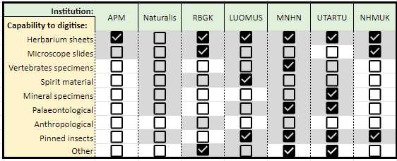
Returned costbooks versus stated capability to digitise from
Legend: Graded shaded = stated capability to digitise. Black tickbox = completed costbook returned for that category.
RBGK 'Other' = fungi collection. MNHN 'Herbarium sheets' = two workflows (day-to-day digitisation in the museum, and Recolnat project workflow). MNHN 'Other' = marine invertebrates collection. UTARTU 'Other' = lichens and fungi. NHMUK 'Pinned insects' = two workflows (standard workflow with label removal, and ALICE workflow with label remaining in situ).
Of the eight collection types, two have widely established, mature workflows with costs: herbarium sheets and pinned insects. Herbarium sheets have long been ahead of the other preservation/collection types in terms of established methodologies and protocols with international projects such as the JSTOR Global Plants Initiative (
GBIF “preserved specimens” mapped to natural history collection types: The results of a search of the GBIF data portal carried out on 26th November 2019 to ascertain the proportion of preserved specimens falling into each of the major natural history collection types. Search filtering on the term “preserved specimen” yielded a total of 166,367,960 results. Within these results, the major taxonomic groups can be mapped to collection types as shown.
|
Main natural history collection types |
Percentage of GBIF preserved specimens |
|
Animalia Arthropoda Insecta Chordata Aves Actinopterygii Mammalia Mollusca |
47% 24% 21% 17% 5% 4% 3% 4% |
|
Plantae |
46% |
|
Fungi |
4% |
As can be seen from Fig.
A recent ICEDIG study of state-of-the-art approaches to mass imaging of liquid samples, which covers spirit material, concluded that mass digitisation for these collections is currently unfeasible hence the lack of mature workflows (
Microscope slide digitisation was also the subject of an ICEDIG report. While mass imaging approaches have been developed and shared (
The remaining collection types (Anthropological, Palaeontological, Mineralogical and non-insect Invertebrates) were not included in the scope of ICEDIG digitisation research. While non-insect invertebrates are a major collection type, they were accidentally omitted from the scope of
3.1 Establishment costs
As illustrated in Table
Establishment costs (PPS) for herbarium sheet and pinned insect digitisation capabilities.
|
Herbarium line (n = 7 stations) |
Pinned insect line (n = 5 stations) |
|
|
Minimum equipment cost |
€12,937 |
€4,109 |
|
Maximum equipment cost |
€40,670 |
€40,816 |
|
Average cost |
€35,593 |
€17,729 |
|
Median cost |
€35,447 |
€8,808 |
Establishment costs are highly variable as is their effect in overall annual digitisation costs. Detailed breakdowns and descriptions of equipment purchased were not given for most of the costbooks, whereas in several cases some additional information was given indicating that costs also included computers, printers and other ancillary equipment. This makes it hard to understand what the costs really cover and the variations between institutions. Because of this the numbers mask differences in the kinds of equipment purchased so comparisons can be made only cautiously.
In the case of herbarium digitisation, the gathered costs mainly relate to equipping a single workstation; yet in one case it is known that an automated conveyor system was included, and in another case, it is known that a high-capability/resolution scanner was purchased. Nevertheless, the average and median costs are similar, with a range of €26,000 – €38,000 PPS as a typical workstation cost. When an integral conveyor system is included, the cost is higher.
Pinned insect lines show a greater variability across the range of reported establishment costs. Insect lines are one area subject to much recent innovation in attempts to increase throughput, and thus a greater variety of novel equipment solutions have been purchased and tried. It’s not possible to give a typical cost for establishing a pinned insect line, except to say that for static (low throughput) solutions the equipment costs are typically low – basically a few thousand PPS for camera(s) and lighting, whereas introducing automation via a conveyor system for higher throughput substantially increases costs (by an order of magnitude).
For several digitisation capabilities, insufficient data was returned to give any credible picture of establishment costs for other collection categories. One outlier worthy of note is a setup composed of a specialised fluorescence/brightfield slide scanner and research microscope for digitisation of microscope slides. This cost more than €150,000 PPS.
In common across all institutions and regardless of digitisation workflow/capability is the observation that establishment costs focus almost solely on equipment purchase and to a lesser extent on costs of acquisition and upgrade. Few non-equipment elements of the expected costs of establishment – such as building/workspace renovation costs, new furniture, electrical work, etc – were reported. This suggests either that such costs are not frequently incurred or (more likely) that such costs are unknown or cannot be accurately accounted for after the fact.
Space requirements for equipment range from 10m2 – 65m2 with average and median of 29m2 and 25m2 respectively. 15m2 – 20m2 seems to be a typical amount of space needed for these kinds of digitisation facilities, with conveyor systems needed larger spaces.
Finally, depreciation periods for such equipment are typically stated as 5 or 7 years, indicating that respondents consider this to be a reasonable lifetime for such investments (even if actual lifetimes are sometimes longer).
3.2 Fixed costs
Establishment costs are one-off costs, normally funded out of capital budget, infrastructure development or project grants. Depreciation is therefore used as an element of the fixed costs calculation to give a truer reflection of the actual cost of digitising specimens. Depreciation costs vary, depending on the original establishment cost and the chosen depreciation period.
Fixed costs are unrelated to the volume of specimens digitised. No matter how high or low are the rates of digitisation, fixed costs remain the same. Table
|
Institution |
Herbarium line |
Pinned insect line |
|
APM |
14.9% |
- - |
|
LUOMUS |
15.6% |
42.8% |
|
MNHN |
73.8% (inhouse) 15.2% (ReColNat) |
65.4% |
|
NHMUK |
98.8% |
100% (ALICE) 100% (Standard) |
|
RBGK |
46.2% |
- - |
|
UTARTU |
96% |
16.1% |
|
Herbarium line (7 stations) |
Pinned insect line (5 stations) |
|
|
Depreciation |
7.6% |
10% |
|
Space charge |
7.6% |
6.3% |
|
Fixed staff cost |
53% |
50.4% |
|
Overheads |
27.2% |
29.9% |
|
Other costs |
4.7% |
3.3% |
Fixed staff cost made up the largest percentage of total fixed costs. Some institutions factor staff into fixed costs (e.g. NHMUK where digitisation staff are largely on long term contracts) while others consider it a variable cost depending on the finance structure that supports the role. Every institution reported fixed-term staff except for RBINS and every institution reported variable cost staff except for the NHM. Among the institution that report fixed cost staff, the average number of staff was 0.84 with a maximum of 2.5 and the total annual labour cost ranged from €1,798 – €124,025 PPS, the highest case of which was MNHM’s outsourced workflow for ReColNat.
Labour was considered a factor in both fixed and variable costs. When considering the impact of staff costs on overall annual cost, it is important to note that some institutions may have entered the same staff member across multiple sheets, thus ‘double counting’ both the number of staff and the cost associated with that staff. This should be taken into consideration when considering institution-level costs and, in future developments of this analysis, should be re-assessed.
3.3 Variable costs
There were two sources of variable costs that were measured in this analysis – variable cost labour and the cost of consumables. Table
|
Institution |
Herbarium line |
Pinned insect line |
|
APM |
85.1% |
- - |
|
LUOMUS |
84.4% |
57.2% |
|
MNHN |
26.2% (inhouse) 84.8% (ReColNat) |
34.7% |
|
NHMUK |
1.2% |
0% |
|
RBGK |
53.8% |
- - |
|
UTARTU |
4% |
83.9% |
Where labour is considered a variable cost, it makes up a significantly larger percentage of variable costs than consumables (although the potential for double-counting should be taken into consideration). Labour costs were calculated by number of staff, their average gross monthly salary and the length of their working week. The average number of variable-cost staff (excluding the NHM who reported none) among the remaining workflows was 1.54, with a maximum of 4, indicating that it may be more feasible for many institutions to employ variable-cost staff than a team of full-time fixed-cost staff.
Using and treating labour as a variable cost implies that the cost of digitisation can more easily be pushed downwards, as these costs are only be incurred when digitisation is taking place – unlike where labour is treated as a fixed cost, meaning that the labour is being paid for even when no digitisation is taking place.
However, in practice labour is rarely fully ‘elastic’ and unless an institute can easily switch staff between digitisation and other tasks there are costs in redeployment, recruitment and training.
For the fix institutions with variable-cost staff, total annual fixed labour cost ranged from €18,727 – €123,264 PPS. One of RBGK’s workflows included national insurance payments and superannuation into their calculations and was removed from this analysis due to its incomparability to other workflows.
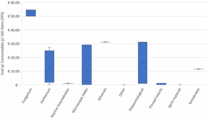
The cost for consumables per batch of 100 objects (single specimens or containers) ranged from zero to €54.49 PPS. The specific consumables used for each project were not named in every case, so it is not possible to identify precisely what the costs are or the reason for this wide range in consumables cost. The two reported cases of fungarium had a much higher cost for consumables than other specimens (Fig.
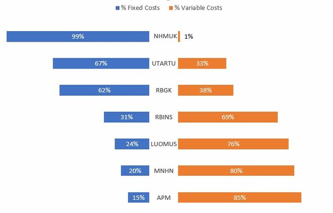
3.4 Fixed versus variable costs
Fig.
|
Institution |
Herbarium line |
Pinned insect line |
||
|
Fixed costs |
Variable costs |
Fixed costs |
Variable costs |
|
|
APM |
14.9% |
85.1% |
- - |
- - |
|
LUOMUS |
15.6% |
84.4% |
42.8% |
57.2% |
|
MNHN |
73.8% (inhouse) 15.2% (ReColNat) |
26.2% 84.8% |
65.3% |
34.7% |
|
NHMUK |
98.8% |
1.2% |
100.0% (ALICE) 100.0% (Standard) |
0.0% 0.0% |
|
RBGK |
46.2% |
53.8% |
- - |
- - |
|
UTARTU |
96.0% |
4.0% |
16.1% |
83.9% |
3.5 Throughput
Direct comparison of the reported rates of digitisation between institutions is not possible as each has different setups and team compositions, as illustrated in Table
Workflow type and staff counts to operate.
Legend: [<fixed staff count>, <variable staff count>]
Note: Except for MNHN’s automated ReColNat workflow, which is outsourced, all other workflows run in-house.
|
Institution |
Herbarium line |
Pinned insect line |
|
APM |
Manual [0,1] |
|
|
LUOMUS |
Semi-automated [0.1,3] |
Semi-automated [0.1,1] |
|
MNHN |
Manual (inhouse) [1,1] Automated (ReColNat) [3,3] |
Manual [0.8,3] |
|
NHMUK |
Manual [1.12,0] |
Semi-automated (ALICE) [1.12,0] Semi-automated (Standard) [1.12,0] |
|
RBGK |
Manual [2.5,2] |
|
|
UTARTU |
Manual [0.2,0] |
Manual [0.1,1] |
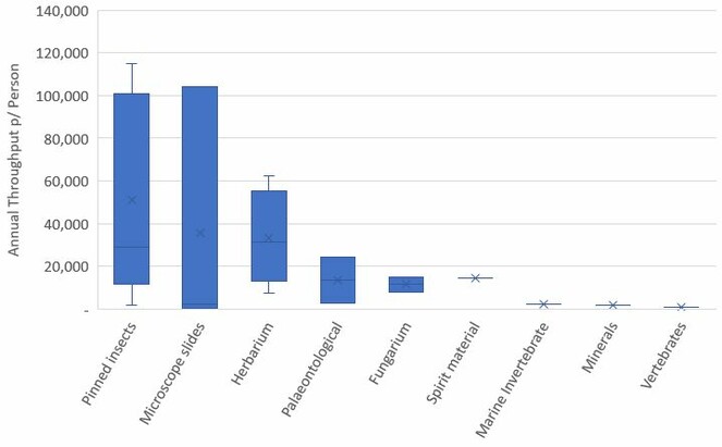
These differences in workflow and the level of capture can be seen in the throughput within specimen groups. After removing the single case of automated outsourcing due to its exponentially higher throughput, the remaining 22 workflows showed a wide range of throughputs where more than one case was reported, particularly for microscope slides and pinned insects (Fig.
Institutions also vary in the number of staff dedicated to digitisation, ranging from 0.1 to 4.8 people. As labour makes up the largest percentage of digitisation costs, it is important to understand labour’s impact on throughput. Contrary to expectations, a larger staff did not necessarily result in a linear increase in throughput. (Fig.
Herbarium specimens showed a slight association between team size and throughput. However, the throughput of pinned insects varied widely on teams of one from 1,737 to 114,700 specimens annually, with the largest team of 3.8 returning the smallest throughput. While semi-automated processes did tend to show a higher throughput, the two cases of manual processes for pinned insects showed a throughput of 21,818 and 1,736. While the one case of an herbarium semi-automated workflow did yield one of the highest throughputs (52,800), the highest was a manual workflow (62,400).
These differences may be due to the depth of information collected in the digitisation process. While it is hard to make direct comparison with workflows, both LUOMUS and NHMUK have developed high throughput workflows for pinned insects (
3.6 Per Item Time
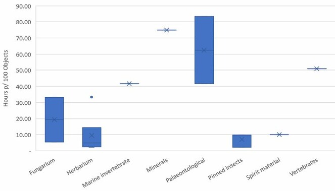
The time required to digitise a batch of 100 objects (single specimens or containers) is affected by multiple factors, including: layout of the institutions, storage facilities, equipment available, etc. There were 18 reported cases of time spent across all specimen types –NHM and RBINS did not provide any time data. The median hours spent digitising 100 objects was 9.88 and ranged from 2.10 to 217.67. RBGK’s microscope slides, the high outlier, are exponentially more time consuming than any other specimen type and was removed from further analysis.
The two palaeontological cases had a wide range, with one requiring 41.67 hours per 100 objects and the other double at 83.33 (Fig.
Time was also estimated for each stage of the digitisation process – curation, image capture, image processing, data capture and preservation. In general, curation was the most time-consuming step in the process across most projects and specimen types (Table
|
Institution |
Country |
Specimen Type |
Curation |
Image Capture |
Image Processing |
Data Capture |
Preservation |
|
UTARTU |
Estonia |
Minerals |
50.00 |
8.33 |
8.33 |
8.33 |
- |
|
UTARTU |
Estonia |
Palaeontological |
50.00 |
8.33 |
16.67 |
8.33 |
- |
|
MNHN |
France |
Vertebrates |
30.00 |
10.00 |
1.67 |
8.33 |
0.83 |
|
MNHN |
France |
Marine invertebrate |
15.83 |
14.17 |
2.50 |
8.33 |
0.83 |
|
MNHN |
France |
Palaeontological |
15.83 |
14.17 |
2.50 |
8.33 |
0.83 |
|
UTARTU |
Estonia |
Fungarium |
6.67 |
6.67 |
6.67 |
6.67 |
6.67 |
|
UTARTU |
Estonia |
Herbarium |
6.67 |
6.67 |
6.67 |
6.67 |
6.67 |
|
MNHN |
France |
Pinned insects |
4.33 |
1.67 |
1.67 |
2.00 |
0.08 |
|
MNHN |
France |
Herbarium |
3.33 |
0.83 |
0.83 |
2.50 |
0.63 |
|
RBGK |
UK |
Fungarium |
2.83 |
2.00 |
0.15 |
- |
0.33 |
|
LUOMUS |
Finland |
Spirit material |
2.00 |
2.00 |
2.00 |
2.00 |
2.00 |
|
MNHN |
France |
Herbarium |
1.75 |
0.17 |
0.02 |
0.15 |
0.08 |
|
UTARTU |
Estonia |
Pinned insects |
1.67 |
3.33 |
0.83 |
3.83 |
0.03 |
|
LUOMUS |
Finland |
Pinned insects |
1.03 |
0.67 |
- |
0.33 |
0.07 |
|
RBGK |
UK |
Herbarium |
0.92 |
0.70 |
0.15 |
0.20 |
2.47 |
|
APM |
Belgium |
Herbarium |
0.25 |
1.33 |
- |
4.00 |
- |
|
LUOMUS |
Finland |
Herbarium |
0.17 |
0.83 |
0.17 |
1.33 |
0.17 |
3.7 Per Item Cost
In order to assess the cost per item, an RBGK project that included national insurance and pension payments in their cost analysis and their case of microscope slide digitisation which had an exponentially higher cost per item than all other cases (€381.26 PPS) was excluded, as well as an UTARTU case that did not provide cost data. This left 19 cases.
The median cost per item across all cases was €2.10 PPS, ranging from €0.53 PPS to €34.22 PPS. Again, the range between the two cases of palaeontological digitisation proved to be the widest while pinned insects and herbarium were relatively consistent. The median cost per item for herbarium was €2.78 PPS and for pinned insects was €1.06 PPS (Fig.
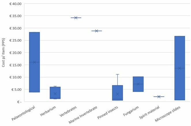
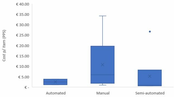
In the two cases where the digitisation process was fully automated – MNHN’s outsourced ReColNat workflow and UTARTU’s palaeontological collection – cost per item was reduced considerably (Fig.
|
Automated |
Semi-Automated |
Manual |
|
|
Median Monthly Throughput per Person |
7,902 |
5,837 |
1,200 |
|
Median Cost per Item |
€2.49 |
€.97 |
€5.94 |
3.8 Size and method
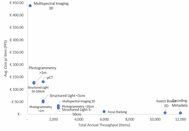
While six out of seven institutions returned costbooks categorized by specimen type, RBINS return costbooks categorized by method of digitisation and size of the item being digitised. While this makes it difficult to compare with other institutions, it does provide insights into different aspects of digitisation costs by showing which methods of digitisation are more costly than others.
For example, 3D imaging is the most expensive digitisation method and with a very low throughput offset by the quality of the image captured. Transcribing metadata and 2D photo captures of insect boxes are the least expensive and have the highest throughput. Interestingly, µCT scanning has the highest annual total cost because of high fixed depreciation costs for X-ray equipment (€63,571 a year). However, the average cost per item remains relatively low because µCT achieves a throughput that offsets the increased costs. Fig.
3.9 Transcription Costs
In conjunction with this costbook analysis,
The minutes per item for transcription ranged significantly from ~30 seconds to up to 41 minutes to fully transcribe label data on a specimen. This large is due to the range of information that is included in the transcription process, the method used and the amount of quality assurance required. For example, georeferencing adds significantly to the time required for transcription, particularly if the label includes only vague location description. Some case studies reported that they did not include georeferencing because of limitations on either time or funding.
Some of the case studies provided examples of either outsourcing transcription to a service like Alembo, using a crowdsourcing platform like DigiVol or testing an automation tool like Google Vision. In each of these cases, staff resources were saved by not requiring museum labour resources for the actual transcription. However their were, in each case, time and money trade-offs for the increased need for project management, volunteer recruitment, quality checks and/or development resources needed to carry out the project.
The analysis showed that, consistent with the other digitisation components studied in this report, time and cost can vary significantly depending on collection type, staff resources and method deployed.
4. Discussion
The process of data collection for this study revealed complexities in gathering and assessing accurate cost data. First, there were inconsistences in how workflows are named and categorised. In asking for the specimen type, one institution used ‘mycological’ and another used ‘fungarium’ to describe digitising their fungi collection. The first institution categorised this workflow as a herbarium collection and the latter as ‘Other’. This is indicative of limitations and inconsistencies in the terminologies used to describe collections and, subsequently, how they are categorised and analysed. For the purposes of this study, both were categorised as ‘fungarium’.
An inconsistent approach to describing collections of physical specimens is a wider challenge that the natural science community is attempting to address. While many efforts have been made within and across institutions to generate and share collection descriptions data, the lack of common standards, data model and vocabularies remain a significant barrier to making these datasets comparable and interoperable. The terminology issues described above are a result of this lack of consistency and standardisation across institutional practices.
The Biodiversity Information Standards organisation TDWG, (https://www.tdwg.org) is developing a new Collection Description data standard to support harmonisation of data across these various resources, and using collection descriptions to underpin specimen digitisation activities is one of the major use cases for the standard (
Secondly, different workflows were broken out into separate cost books. However, some institutions recorded the same number of employees across multiple workflows and, in some cases, the same time and costs associated with different collections. It is unclear if these were separate but identical costs that could thus be summed, or if they were the same costs and thus a double counting of the same data.
ICEDIG recommends working towards harmonisation of approaches to costing digitisation. This will become more important as various kinds of decision about digitisation are made e.g., prioritisation, allocation of certain types of mass digitisation to specific facilities, budgeting, authorization of on-demand digitisation requests, etc.
For categories of collection where digitisation has been carried out by a significant number of institutions, it’s reasonable to look at the spread of costs achieved and to focus on transferring knowledge and learning points from those institutions of low cost to those where costs are higher, in an effort to increase cost efficiencies.
For categories of collection where digitisation has been carried out by only a few institutions, the aim should be to spread best practice to institutions embarking on digitisation of these categories as a means to avoid repeating past mistakes and accelerating progress towards efficient (low-cost) digitisation across institutions in those categories.
Recommendations on capital equipment choices, whilst probably appropriate for DiSSCo to give guidance on, is out of scope of the present document.
Based on this costbook exercise an ambitious baseline for mass digitisation of pinned and herbarium sheets would be less than €0.50 PPS per item. This is based on a very limited sample of institutions and workflows so should be taken as indicative only. There is not enough data to make suggestions on baseline costs for digitising other specimens but in order to meet DiSSCo’s mass digitisation goals we need to encourage and support continuous improvements to drive that cost down and to increase throughput without increasing per item cost. In practice, also, digitisation projects vary widely, and the degree of data captured should relate to the project aims – where more data is most appropriate (e.g., a key project aim is full georeferencing or some kind analytical treatment of an object) it may well be appropriate to accept a higher baseline cost.
5 Recommendations
In addition to the discussion points above we recommend the following:
-
Focus on harmonisation of costing approach – standardisation of the methodology for gathering and reporting costs. We recognise that many institutes will have difficulty gathering and providing detailed cost information and that a simpler costing approach may be required.
-
Focus on cost improvements (efficiencies) – recommend setting a target mass digitisation cost (per specimen) for different types of collection. If we had to set it today, what would we set it at? A strong focus on cost improvement would be one of several means of accelerating progress in mass digitisation.
-
Consider how we can transfer best practice between institutes and digitisation teams.
-
Track digitisation costs over time as standard - we currently have limited data on digitisation costs and if more institutes started recording this data we could better identify effective and ineffective practice.
5.1 Expanding scope of gathered costs
Anthropological, Palaeontological, Mineralogical and non-insect Invertebrates collections were not included in the scope of ICEDIG digitisation research. While non-insect invertebrates are a major collection type, they were erroneously omitted from the scope of
5.2 Other considerations
The costbook work in ICEDIG will be inherited and expanded upon by the DiSSCo Prepare project, specifically in Tasks 4.1 and 4.2, the “Costbook for DiSSCo” and “Cost model for charging services”, and their corresponding reports.
While not directly working on a costbook, SYNTHESYS+ will be gathering and assessing cost data as part of the new Virtual Access workpackage (
In the subsections that follow, we offer some further considerations that other projects in the DiSSCo Programme portfolio should take into account but they apply to any organised large scale digitisation of collections.
5.2.1 Future development and maintenance for collecting new data
The current method for collecting, aggregating and analysing data from different institutions, based on completing pre-formatted spreadsheet templates becomes cumbersome when the number of responding institutions increases and quantities of data increase. Significant manual work is involved both for the institutions in filling templates and for analysts to work with the returned data.
An alternative approach to spreadsheets
As we noted when considering implementation of the costbook template (see section 2.6), alternative approaches are available and should be considered. One such is Airtable (https://airtable.com/), a modern and flexible spreadsheet-database hybrid offered ‘as-a-service’ that allows teams to collaborate in the contribution and analysis of data. With both free and paid options, Airtable presents like a cloud spreadsheet (like Google Sheets) but also supports linking between sheets to form basic relational data structures, providing some of the benefits of a database. Table
|
Pros |
|
|
Cons |
|
Regardless of whether Airtable is the specific correct product to adopt, the key learning point is that reliance on old-style spreadsheet products, distributed and managed as files among participants is no longer necessarily the most flexible, efficient or sustainable approach to gathering, collating, analysing and using actual cost information. The recommendation here is that DiSSCo should consider alternatives to the Excel/Google spreadsheets approach for modern management of cost information. However, any change from using commonly used software to a new webform or database will require sufficient support to ensure it is fit for purpose.
Recommendation: DiSSCo must evaluate and adopt modern alternative(s) to traditional spreadsheet approaches for the management of cost information.
Standardising currency
Several currencies have been used throughout the cost gathering and analysis work. The NHM UK entered their data in £ sterling. Other institutions entered their data in € euros. For summation, conversions were done to the EC’s PPS Purchasing Power Standard. However, we failed to foresee that we might want to do some analytical calculations, for example stating specific cost components, such as depreciation as proportions (%) of a total annual cost. This involves going back and re-manipulating specific parts of the data.
A more helpful approach would be to convert from the currency used for data entry to PPS for each data item entered, at the time of entry. This would facilitate the kind of calculation exampled above.
Recommendation: In cost gathering, budgeting and accounting, DiSSCo should convert, at the time of data entry from the currency of data entry to the standard currency used for accounting purposes.
5.2.2 Sharing best practice
As we noted in the results and analysis, there are clear differences in costs that are most likely a consequence of the differing workflow approaches adopted by different institutions. Constant innovation leads ultimately to either/both higher throughput efficiencies and/or lower costs.
It is evident from anecdotal comments received during the task that practices for recording and breaking out costs, levels of detail of cost records and maturity of accounting for work vary considerably among the responding institutions.
Two elements to communicate best practices about:
- Best practice accounting procedures so that quality and level of detail/accuracy of costing data improves
- Innovations that lead to higher efficiencies/throughputs and lower costs
How then should DiSSCo distil, promote and support dissemination of best practices from established workflows in institutions with high efficiencies and low costs to other institutes that might benefit?
5.2.3 Treating costs separately from charges
Costs must be treated separately from charges. A cost model is not the same as a charging or business model, and the latter is not part of the present task. Nevertheless, in the end, cost calculations cannot be considered in isolation from a business/charging/organisational model, because of the influence of DiSSCo governance decisions and policy on requirements for digitisation, data access and availability. Digitisation can be required to a certain level. Some data may be more immediately available than other data, according to scientific demand and difficulty to retrieve (faster and easier versus slower and more time-consuming).
In-depth analysis of potential business models is described in
Any business model must, however, take both depreciation and amortization into account.
5.2.4 Depreciation and amortization
Depreciation of equipment
Depreciation is the process of allocating the capital costs of a tangible asset (such as digitisation equipment or storage systems) over time. It’s a measure of how much of the value of an asset has been consumed to a point in time (usually, the end of an accounting period). Note though, that usage of such equipment can usually extend well beyond the depreciation period. Depreciation is well understood and, especially for IT infrastructure, is typically allocated over three or four years using a straight-line method (i.e. the same amount in each year).
Depreciation is used in statutory accounting for matching costs against income and hence for calculating annual profit or loss. Its use in management accounting (as considered here) is as a means of reflecting the true cost of digitising specimens in years following those in which a digitisation facility was established.
Amortization of DiSSCo data
Amortization is the process of allocating the costs of an intangible asset such as data over time (its ‘useful life’). The purpose is to match the costs of creating and maintaining data to the value earned from using that data. Or to put it another way, to ensure that expenses are not incurred in maintaining data with no useful value. Like depreciation, accounting for amortization in multi-year business plans for digitisation is good practice. Because of the multi-stakeholder characteristics of the DiSSCo governance and business model, this is a topic DiSSCo must pay attention to – however this is an area of high complexity where evidence is likely to improve over time.
Accounting for amortization in DiSSCo must match the expense of acquiring, preserving and maintaining ‘FAIR’3 digitised specimen/collection data with the value of the use that data receives over time, usually in a linear fashion over the period of ‘useful life’. Such value, however, can be hard to measure in financial terms - the value of research, education/training and other uses is not usually measured financially, partly because there are no accepted standard methods for doing so. Proxy measures can be useful; such as the number and impact of scientific publications achieved from having the data available; or the number and value of new research grants enabled by digitisation. Such metrics must be tracked from an early stage by the Digitisation Dashboard application.
We know the useful life of physical specimens in collections can easily be measured in decades or hundreds of years. But we also know the usefulness of both individual specimens and collections of specimens varies enormously, according to the scientific and societal questions of the day. What is the useful life of Digital Specimens and Digital Collections? For arriving at a practical basis for valuation and amortization, we must model several scenarios where amortization periods are set at say, 10, 25 and 50-year intervals.
In future, large-scale (mass) and more ‘bespoke’ digitisation can both be operated more frequently on a digitisation-on-demand basis, i.e. fulfilling demands for specimen information by immediately digitising it and making it available on request on efficient digital platforms. There are arguments that this is more cost-effective: adapting words from elsewhere5, we could say that immediate digitisation is better than storage, meaning that it is more cost-effective to rapidly digitise and deliver only what is requested than to systematically and slowly digitise and store everything that is collected. In practice, however, experience to date of systematic digitisation is that its benefits are not always predictable – there is a strong element of serendipity e.g. in use of collections data alongside other data via aggregators; and there can be ‘critical mass’ of data for certain kinds of research (‘big data’ approaches). Sometimes, demand does not exist until data is made available, and data availability can enable new research paradigms and stimulate future demand. NHMUK’s Digital Collections Programme, for example, track citations of digital specimen data – these data have not been created on demand, but the trend in the growth of usage (and therefore benefit/impact) is increasing year on year.
Once digitised, the value of specimen data does not decay quickly. Indeed, the value can even be increased as digitised specimen data is improved and supplemented with links to other information. There are costs associated with this. First, the costs of digitisation; second, the key cost of storage/preservation/serving over long time periods; and third, additional costs associated with data improvement and supplementation. There must be enough steady and measurable benefit over long periods into the DiSSCo business model to balance costs. An additional complexity is across what ‘body’ of data it is meaningful or accurate to apply amortization– the ‘value’ or benefit of data tends to increase in the context of other data, whether through an increase in the size of the same dataset; additional data from related collections datasets; or data from other sources and of other types/content e.g. climate data. While each digitisation project may look at their own dataset for amortisation and to estimate costs, the benefits and value do not accrue in isolation. Thus, the approach towards amortizing costs of data for DiSSCo must be examined very carefully and kept under review over time.
6. Conclusions
Considering the complexities of the digitisation process, and its variability among institutions and between different types of collections, we conclude that time spent is an essential parameter informing costing information. Other key parameters are labour rates, consumables and fixed cost elements such as heating and lighting, space rental, etc. Actual costs vary from one institution/country to another and our template offers calculators based on simple inputs. Gathered costs can be normalised to take account of different purchasing power of money in different countries.
Optimal digitisation cost is achieved when the volume and availability of specimens ready for digitisation matches the capacity of the digitisation facility. Having enough specimens ready means the digitisation capacity can be effectively utilised and the highest throughput can be achieved, thus leading to the lowest cost (notwithstanding other factors contributing to cost and the assumption that the digitisation facility is dimensioned sufficiently for the task). Too few specimens ready means the capacity is underutilised, meaning higher cost per specimen.
What an institution wants to know is: When can certain kinds of digitisation be achieved for specific levels of investment? When does it become practical/economic to start digitising a collection? What does it cost to invest for digitisation and to reach a certain level for a collection?
The gathered cost information begins to inform answers to such questions. We have made several recommendations to be carried forward elsewhere in the DiSSCo Programme e.g., as specific work items in the DiSSCo Prepare project, for consideration by the DiSSCo Coordination and Support Office and the DiSSCo General Assembly.
Acknowledgements
We express our thanks and acknowledgement to the following individuals who assisted with this report and the underlying data:
-
Hannu Saarenmaa (UH), Ana Casino (CETAF), Xavier Vermeersch (CETAF), Karsten Gödderz (CETAF), Luc Willemse (Naturalis), Michel Guiraud (MNHN), Agnes Wijers (PIC) and Jeroen Bloothoofd (PIC) for contributions towards conception, design and review of the costbook template.
-
Lousie Allan (NHM) for attempting the completion of a trial costbook sheet to help us iron out difficulties.
-
Quentin Groom (APM), Mathias Dillen (APM), Anne Koivunen (LUOMUS), Kari Lahti (LUOMUS), Sarah Philips (RBGK), Lousie Allan (NHM), Veljo Runnel (UTARTU) and Vanessa Demanoff (MNHN) for filling and returning 22 completed templates.
Grant title
ICEDIG – “Innovation and consolidation for large scale digitisation of natural heritage”, Grant Agreement No. 777483
Author contributions
Authors:
Alex Hardisty: Conceptualization, Data Curation, Formal Analysis, Investigation, Methodology, Visualization, Writing – Original Draft, Writing – Review & Editing. Laurence Livermore: Conceptualization, Data Curation, Formal Analysis, Writing – Original Draft, Writing – Review & Editing. Stephanie Walton: Data Curation, Formal Analysis, Validation, Visualization, Writing – Original Draft. Matt Woodburn: Software, Writing – Original Draft. Helen Hardy: Writing – Original Draft, Writing – Review & Editing.
Contribution types are drawn from CRediT - Contributor Roles Taxonomy.
References
-
A Novel Automated Mass Digitisation Workflow for Natural History Microscope Slides.Biodiversity Data Journal7(e32342). https://doi.org/10.3897/BDJ.7.e32342
-
Technical capacities of digitisation centres within ICEDIG participating institutions.Research Ideas and Outcomes6https://doi.org/10.3897/rio.6.e55522
-
ALICE, MALICE and VILE: High throughput insect specimen digitisation using angled imaging techniques.Biodiversity Information Science and Standards3https://doi.org/10.3897/biss.3.37141
-
Provisional Data Management Plan for DiSSCo infrastructure. Deliverable D6.6.Zenodo. https://doi.org/10.5281/zenodo.3532937
-
Conceptual design blueprint for the DiSSCo digitization infrastructure - DELIVERABLE D8.1.Research Ideas and Outcomes6https://doi.org/10.3897/rio.6.e54280
-
SYNTHESYS+ Virtual Access - Report on the Ideas Call (October to November 2019).Research Ideas and Outcomes6https://doi.org/10.3897/rio.6.e50354
-
Five task clusters that enable efficient and effective digitization of biological collections.Zookeys209:19‑45. https://doi.org/10.3897/zookeys.209.3135
-
Towards a Global Collection Description Standard.Biodiversity Information Science and Standards3https://doi.org/10.3897/biss.3.37894
-
Digitise This! Innovation in Digitisation Initiatives within Australasian Herbaria.Biodiversity Information Science and Standards2(e26077). https://doi.org/10.3897/biss.2.26077
-
SYNTHESYS+ Abridged Grant Proposal.Research Ideas and Outcomes5https://doi.org/10.3897/rio.5.e46404
-
Design of a Collection Digitisation Dashboard.Zenodohttps://doi.org/10.5281/zenodo.2621055
-
State of the art and perspectives on mass imaging of liquid samples.Zenodohttps://doi.org/10.3897/zookeys.209.3135
-
A cost analysis of transcription systems.Research Ideas and Outcomes6https://doi.org/10.3897/rio.6.e56211
-
The FAIR Guiding Principles for scientific data management and stewardship.Scientific Data3(160018). https://doi.org/10.1038/sdata.2016.18
-
Automated Methods in Digitisation of Pinned Insects.Biodiversity Information Science and Standards3https://doi.org/10.3897/biss.3.38260
Supplementary materials
Short VBA procedure for extracting data from multiple Excel template sheets into a flattened structure.
This costbook template contains separate calculators for establishment (upfront) costs, for fixed costs of digitisation and for variable costs. We strongly recommend that before using again, to modify the costbook template to allocate named ranges to cells.
The original 22 responses from six ICEDIG collections-holding institutions (APM, LUOMUS, MNHN, NHM, RBGK, UTARTU).
Thirteen costbooks from RBINS covering technique-based digitisation costs (e.g. µCT, photogrammetry, structured light and multispectral imaging).
Digitisation scenarios can be characterised along two axes: capability and capacity (or scale).
On the capability axis a spectrum of possibilities for the organisation of digitisation ranges from temporary or permanent inhouse facilities to fully outsourced contracts of digitisation undertaken by commercial companies. On all points of the spectrum, there can be various proportions of professional and volunteer digitisers contributing effort and affecting operating costs accordingly.
On the capacity axis, digitisation activities can range from small-scale, one-off bespoke projects to digitise specific specimens, collections or parts of a collection through to large-scale, long-term mass digitisation programmes aiming to digitise complete holdings of an institution. At multiple points on this axis digitisation-on-demand can also range from sporadic one-off digitisations (special cases) to continuous routine requests for digitisation.
At the time of writing the present article there is no citation available for the proposed MIDS standard. Readers are advised to refer to the Biodiversity Information Standards (TDWG) website, https://www.tdwg.org/ and/or corresponding GitHub pages/repositories, https://github.com/tdwg/ for the latest status.