|
Research Ideas and Outcomes : R Package
|
|
Corresponding author: Álvaro Briz-Redón (alvaro.briz@uv.es)
Received: 30 Jan 2019 | Published: 01 Feb 2019
© 2019 Álvaro Briz-Redón
This is an open access article distributed under the terms of the Creative Commons Attribution License (CC BY 4.0), which permits unrestricted use, distribution, and reproduction in any medium, provided the original author and source are credited.
Citation: Briz-Redón Á (2019) SpNetPrep: An R package using Shiny to facilitate spatial statistics on road networks. Research Ideas and Outcomes 5: e33521. https://doi.org/10.3897/rio.5.e33521
|
|
Abstract
Spatial statistics is an important field of data science with many applications in very different areas of study such as epidemiology, criminology, seismology, astronomy and econometrics, among others. In particular, spatial statistics has frequently been used to analyze traffic accidents datasets with explanatory and preventive objectives. Traditionally, these studies have employed spatial statistics techniques at some level of areal aggregation, usually related to administrative units. However, last decade has brought an increasing number of works on the spatial incidence and distribution of traffic accidents at the road level by means of the spatial structure known as a linear network. This change seems positive because it could provide deeper and more accurate investigations than previous studies that were based on areal spatial units. The interest in working at the road level renders some technical difficulties due to the high complexity of these structures, specially in terms of manipulation and rectification. The R Shiny app SpNetPrep, which is available online and via an R package named the same way, has the goal of providing certain functionalities that could be useful for a user which is interested in performing an spatial analysis over a road network structure.
Keywords
R package, spatial statistics, linear networks, point patterns, data curation, R Shiny
Introduction
Spatial statistics studies have been commonly based on geographic structures made of polygons representing an administrative or political division of different order, depending on the size of the region being analyzed and on the specific interest of the researchers. More specifically, the basic spatial units in these studies have ranged from larger (countries or counties) to smaller (cities, boroughs, census tracks, etc.), allowing the employment of the usually available information regarding these kind of population units.
However, last years are bringing a higher number of spatial analysis that are defined over network structures, which allow a better understanding of some spatial point patterns of great interest. Basically, the use of spatial networks has become quite frequent when the events of study actually take place in roads, streets, highways, etc., which oblige to discard most of the areal region of the zone of analysis if an accurate investigation is intended. Therefore, the use of linear networks is really interesting to analyze the spatial distribution of traffic accidents (
Let's review now some basic terminology about linear networks in the context of spatial statistics. A planar linear network, \(L\), is a finite collection of line segments, \(L=\cup_{i=1}^{n} l_{i}\), in which each segment contains the points \(l_{i}=[u_{i},v_{i}]=\{tu_{i}+(1-t)v_{i} : t\in [0,1]\}\) (
A point process \(X\) on a linear network \(L\) is a finite point process in the plane such that all points of \(X\) lie on \(L\) (
Overview of the package
The SpNetPrep package (
The main feature provided by the SpNetPrep package is an interactive application that allows to carry out the complete preprocessing of a linear network that comes from a road structure. First, the user needs to install the package via CRAN (the package is also described in https://cran.r-project.org/web/packages/SpNetPrep/index.html) or GitHub (https://github.com/albrizre/SpNetPrep) through the instruction install_github("albrizre/SpNetPrep") (which requires to call the devtools package). Then, the execution of the function runAppSpNetPrep() in the R console launches the application allowing its full use, which is also possible to be done online following the link https://albriz.shinyapps.io/spnetprep/. If the application is run from the R console, it is necessary to click the option "Open in browser" when it shows, or define "Run external" for the opening of Shiny applications in order to be able to download the modifications performed on the objects uploaded to it.
According to the technical difficulties that the development of a spatial analysis over a linear network implies, the SpNetPrep takes advantage of the R packages leaflet (
Users can obtain a road network of their interest via the OpenStreetMaps (OSM) platform (
When the user is in possession of a road network in a right R format (these formats will be described later), the SpNetPrep application includes a "Network Edition" section that usually would constitute the starting point of the preprocessing phase. At this part of the application, users can introduce their networks in order to delete edges, join vertex to form new edges and create new points that are connected to the preexisting vertex or directly between them. Of course, users that had previously created their road networks with SpNetPrep can use this edition section to make changes on them.
The manual edition (or curation) of a linear network representing a road structure is an important step that must be taken in order to correct possible mistakes (not updated road configurations), remove some undesired parts (pedestrian or secondary roads, depending on the application) and also to simplify some zones of the network whose complexity could obscure the analysis being performed (which is sometimes very notorious in round-abouts or complex intersections).
Furthermore, in view of the difficulties that sometimes can arise when trying to obtain a road network structure, the "Network Edition" section of the SpNetPrep application could also be employed to create a road network from scratch (the user would need to upload a dummy road network of at least one segment within the region of interest). Of course, this would not be a good option if the aim of the user is the creation of a complex road network made of hundreds of kilometers, but it can be a cost-effective option for creating small road networks within an urban area, or even for a long network representing highways or rural roads given its (usually) greater simplicity.
Another important question to take into consideration when working with a linear network structure is its directionality. Depending on the kind of dataset being treated, network direction could be of no interest, but this should not be the case when analyzing traffic-related data. In fact, traffic flow could be dramatically influential for some classical spatial analysis that arise from this kind of data. For example, in order to fit a spatial model to a collection of accident counts at the road segment level (for instance, with the spdep package from
Again, it is not easy, at all, to find the information required to endow a linear network based on a road structure with a directionality. The network structures available in OSM contain some information regarding the direction of the streets and some cartographic platforms include the direction of traffic (measured in angles) at some points of the structure, but, in general, it can be really hard to obtain such information for a road network of your interest. For this reason, the "Network Direction" section of the SpNetPrep application attempts to facilitate the enhancement of a network with this valuable information.
Once the network structure is properly curated and endowed with a direction (if necessary), a point pattern can be formed along the network structure from a dataset containing geocoded information. In the case the information on the location of each event is in the form of a postal address, the R package ggmap (
Then, when the coordinates of the events of interest are already available, regardless of the way they have been obtained, it is time to project them into the linear network. This step can be achieved straight by using the (shortest) orthogonal projection of each pair of coordinates into the linear network, for example with the project2segment function of the R package spatstat (
As a summary, Fig.
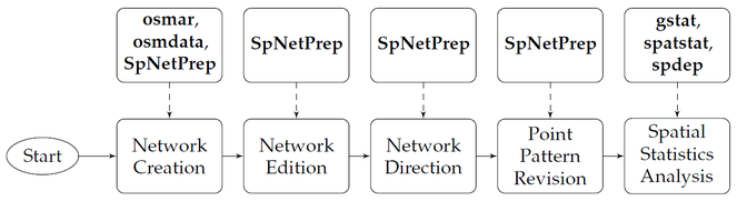
Workflow that describes all the steps that could be carried out in order to perform a spatial analysis on a point pattern that lies on a linear network. Some of these steps which lead to the final statistical analysis may be skipped but, at least, all of them should be considered. The blocks pointing the steps of the process include some of the R packages that would allow to successfully achieve each of them.
Technical issues
The present section includes some notes on certain technical aspects that need to be known in order to benefit from SpNetPrep functionalities.
Linear networks in R
There are two main classes coexisting in R that represent what a linear network is: SpatialLines and linnet. The class SpatialLines belongs to the sp package (
Geographical projections
Coordinate Reference Systems (CRS) are essential to locate entities in space. Concretely, each CRS defines a specific map projection that unambiguously determines the location of every point on the Earth, which makes impossible to deal simultaneously with two geographic objects described in a different projection system. The usual longitude and latitude coordinates, which range from -180º to 180º and -90º to 90º, respectively, correspond to the WGS84 (World Geodetic System 1984) geographical projection. One important characteristic of the WGS84 projection system is that it considers the whole world as a unique zone, that is, a pair longitude-latitude in this CRS system determines only one point of the Earth. However, this situation does not hold for the Universal Transverse Mercator (UTM) projection system, another well known CRS that divides the world into 60 zones whose coordinates are denoted easting and northing in analogy with longitude and latitude (respectively). The use of the UTM system is more convenient for performing statistical analysis given its higher level of accuracy (specially when working with small areas) and also because the coordinates it provides are expressed in meters, which renders very easy to compute distances. The sp package allows to deal with projection systems by means of the CRS class and the proj4string method. The following lines exemplify how to proceed, assuming that wgs84object and utmobject are two sp objects expressed in WGS84 and UTM (zone 30) coordinates, respectively, whose projections had not been established yet in the R environment. Basically, the proj4string assigns a projection system to an sp object whereas the spTransform function changes an sp object's projection from one system to the other.
> CRS_wgs84<-CRS("+proj=longlat +datum=WGS84 +ellps=WGS84 +towgs84=0,0,0")
> CRS_utm<-CRS("+proj=utm +zone=30 ellps=WGS84")
> proj4string(wgs84object)<-CRS_wgs84
> proj4string(utmobject)<-CRS_utm
> wgs84object_transform<-spTransform(wgs84object,CRS_utm)
> utmobject_transform<-spTransform(utmobject, CRS_wgs84)
Working with files in the SpNetPrep application
Format. RDS has been chosen for all the files possibly involved during the use of the SpNetPrep application, which means that inputs and outputs will always be in this R file format. Functions readRDS and saveRDS allow to read and create, respectively, a .RDS file for its use in the application or in the usual R console. On the CRS system, the SpNetPrep application is only ready to accept input files from that are expressed in UTM coordinates. These coordinates are then internally converted into the WGS84 system in order to be usable by the leaflet functions that are employed for making the application work. Consequently, the output files that can be downloaded after the use of any of the sections of the application are also in UTM coordinates, allowing its direct use for statistical analysis if no more preprocessing steps are required. Furthermore, for the "Network Edition" and "Network Direction" parts of the application the inputs are required to belong to the sp package, whereas for "Point Pattern Revision" it is needed to upload an object that has been created with the lpp function of spatstat (more details later). The UTM zone needs to be specified by the user with the proj4string method in the case of the sp objects and typing it on the corresponding text input for the "Point Pattern Revision" section of the application as otherwise the application will yield an error message. In case of trouble during the construction of the input files, the data objects SampleNetwork, SampleDirectedNetwork and SamplePointPattern available in the package can serve as a reference for the sections "Network Edition", "Network Direction" and "SamplePointPattern", respectively, although the first of these data objects also works for the "Network Direction" part. Finally, it is convenient to remark that, even though the application has been subject to the usual debugging tests, the raise of an error could break the application and make users lose their work. For this reason, it is highly recommended to execute and download the changes being performed in the road network or point pattern being used regularly.
Network edition
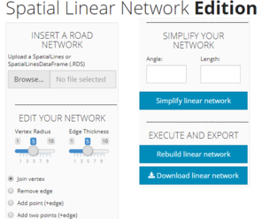
Manual edition of the geometry of a linear network is one of the main purposes of the SpNetPrep application. This process includes the manual rectification of the network, which basically consists of performing edge addition/deletion and vertex addition/deletion. Furthermore, the application provides an algorithm of automatic simplification that reduces network's complexity while accounting for its basic geometric structure, which will be later described. First, the use of the "Network Edition" section of the application is explained.
Application's use
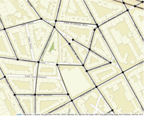
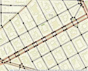
There are four basic actions that can be performed for editing the linear network manually: "Join vertex", "Remove edge", "Add point (+edge)" and "Add two points (+edge)". The user only has to select the more convenient option and proceed intuitively. If "Remove edge" is selected, the click on an edge of the network (anywhere all along its length) serves to mark the edge in red, indicating a removal state. Oppositely, by choosing any of the options "Join vertex", "Add point (+edge)" or "Add two points (+edge)" the user needs to click on two points of the map accordingly to the option being selected. For the "Join vertex" option, two vertex must be clicked, whereas for the "Add two points (+edge)" two points of the map (that are not vertex) have to be clicked. Finally, the "Add point (+edge)" requires that the user clicks on a point and on a vertex of the network (in this order). All these three options that imply the addition of edges (and maybe vertex) to the road network are marked in green. The click of the button "Rebuild linear network" makes this manual editions effective and when the map refreshes the new (edited) road network is available for the user (which can be downloaded by clicking on the button available at the bottom of the application). Now, let's see and example of use of the "Network edition" section of the application (Fig.
Automatic network simplification
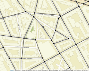
The SpNetPrep package includes a function called SimplifyLinearNetwork, which is also provided in the sidebar panel of the "Network Edition" section of the application, that could be very helpful during the network preprocessing process. This function (which accepts and produces linnet objects) consists in the execution of an algorithm that attempts to automatically reduce network's complexity without altering its basic geometric configuration. The main objective of the algorithm is to merge the pairs of edges of the network that are connected by a second-degree vertex (with only two incident edges) into only one edge. Equivalently, this action means to join two vertex of the network whose path of connection only passes through another vertex of the network. Two are the parameters that control the extent to which this algorithm simplifies the linear network: edge Length and Angle between edges. The tuning of these two parameters allows the user to test several simplifications of the network that imply different levels of conservation of its geometric structure. Both parameters work in the same direction: merging between two edges only produces if their lengths (of both) are lower than Length and if the angle they form is below the value of Angle. The continuous increase of Length and Angle can derive into a very simplified network (with a minimal number of vertex and edges), but this process has the cost of producing a geometric structure much more dissimilar to the original one. More specifically, an analysis on the choice of Length and Angle was performed by using a road network from the city of València (Spain). The Angle parameter was varied from 0º to 90º, whereas Length made it from 0 m to 500 m. The level of simplification achieved with every combination of the parameters was measured in terms of the percentage of second-degree vertex that were removed by merging their two incident edges, which is the objective of the algorithm. The Hausdorff distance (

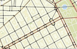
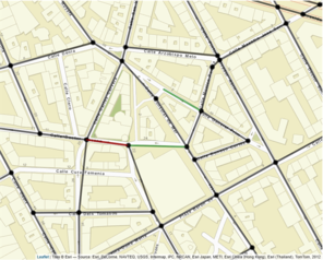
Example of use of the SimplifyLinearNetwork function.
b: Simplified version of the network in a after the application of the SimplifyLinearNetwork function with parameters Angle = 25 and Length = 65
For practical reasons, the use of a combined condition for the Angle and Length parameters is only available in the SimplifyLinearNetwork function of the package, which can be used from the R console. The "Network Edition" only includes an option to perform the simplification procedure with a global value for Angle and Length. At this section of the application, one can alter the values of these parameters and explore the results that produce, but the deeper employment of the algorithm (possibly including the use of the gDistance function to measure geometric dissimilarity) requires to be in the R console.
The following lines include an application of the SimplifyLinearNetwork function to the SampleNetwork available in the SpNetPrep package including both, a unique value for Angle and Length and a combined effect of these parameters (lines headed with a ">" symbol indicate a code instruction, whereas lines missing a ">" are outputs from the R console). The parameters of the SimplifyLinearNetwork function are (in this order): network, Angle, Length and M. As it can be seen, the direct use of Angle and Length leads to a superior simplification of the network (less edges), but some users could be particularly interested in the simplification of pairs of very short edges that meet in a two-degree vertex, which is accounted if the M matrix is used.
> network <- as.linnet(SampleNetwork)
> network
Linear network with 1664 vertices and 2513 lines
> simplified_network_1 <- SimplifyLinearNetwork(SampleNetwork,25,65)
> simplified_network_1
Linear network with 1598 vertices and 2447 lines
> M <- matrix(c(10,60,40,25),nrow=2)
> simplified_network_2 <- SimplifyLinearNetwork(SampleNetwork,M=M)
> simplified_network_2
Linear network with 1639 vertices and 2488 lines
Network direction
The addition of a direction to the road network according to traffic flow may be interesting at some situations. The SpNetPrep package includes a friendly mechanism to achieve this goal, which is explained in the present section.
Application's use
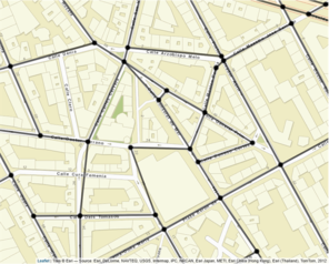
The "Network Direction" section of the application allows the user to endow the network with a direction according to traffic flow, which is facilitated by the presence of arrows indicating this information in the OSM layers. The option "Add flow" enable users to define a flow along the network by simply clicking on the two connected vertex that form the edge they want to give direction to (first click on the origin, second on the end, according to traffic flow). Analogously, "Remove flow" performs the opposite action by removing a direction previously defined, which requires to select the two vertex that form the road segment whose direction is being eliminated (the order of the selections is not important). The function addFlows of the leaflet package overlays a blue arrow on the map when a direction is set, and also erases it when the user decides to undo the defined direction (Fig.
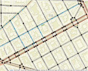
Even though the "Add flow" and "Remove flow" options are sufficient to give direction to the whole network, "Add long flow" and "Remove long flow" attempt to save some time to the user. These functions take advantage of the shortespath function that was used to generate chapter 17 of
Direction information storage
The directionality of the linear network is stored in the form of a data.frame with three columns named V1, V2 and Dir. For each edge of the network, \(i\), V1 and V2 contain the indexes of the vertex of the network that define edge \(i\) (origin and end, according to the way the network was defined or created, which can be meaningless in terms of traffic flow). This data.frame is then attached to the SpatialLines introduced by the user, or added to the existing data.frame if the input is a SpatialLinesDataFrame object. Obviously, users that have already used the "Network Direction" section of the application with a specific road network only have to upload it again in order to make editions to its directionality, and the V1, V2 and Dir columns of the data.frame will be modified accordingly. There are four possible values for the Dir column: 0, -1, 1 and 2. A value of 0 indicates the absence of a direction for an edge, 2 means double way direction, 1 that direction exists from vertex in column V1 to vertex in column V2 and -1 just the opposite (from vertex in V2 to vertex in V1). For example, the following lines include an example of such a data.frame, which describes the minimal linear network (with five edges and six vertex) represented in Fig.
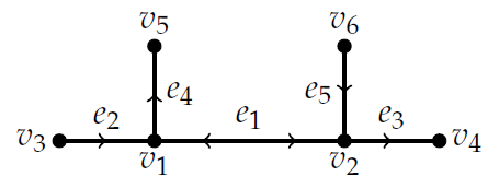
V1 V2 Dir
1 2 2
1 3 -1
2 4 1
1 5 1
2 6 -1
Taking this information into account, users can establish neighbouring relationships between the road segments of their networks that respect traffic flow (employing functions from the spdep package, for instance) or compute distances between points that really represent the way vehicles move along the network.
Point Pattern Revision
Finally, the SpNetPrep appliaction provides the possibility of visualizing and manipulating a point pattern that lies on a road network. This section gives details regarding the features of the package on this issue.
Application's use
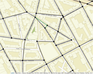
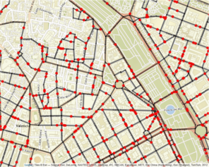
A point pattern that lies on a linear network can be created in R with the lpp function of the spatstat if a spatial point pattern (ppp class) and a linear network object (linnet class) are available. The use of the function marks from the same package allows to add several informative variables to each point of the pattern. It is always useful to have the possibility of visualizing such a point pattern, which can be done with the "Point Pattern Revision" section of the SpNetPrep application keeping the default option "Explore pattern" (if the pattern is marked, the values of the first ten marks, following the definition of the object, are shown when clicking each event). First, visualization usually provides a better understanding of the point pattern which can condition the posterior statistical analysis, but also allows to check that the creation of the point pattern on the linear network produced correctly. For illustrating this section of the application, Fig.
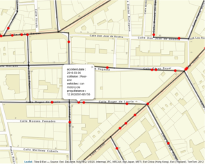
Edition of the point pattern
It was already mentioned in the overview section of the paper that the automatic creation of a point pattern that lies on a linear network in R implies the orthogonal projection of a collection of geocoded events into the network. This operation generally leads to an accurate representation of the observations, but it can produce some misplaced events along the road network. As it is suggested in Fig.
Summary
This paper has presented the main functionalities and purposes of the SpNetPrep R package. Mostly based on a Shiny application that makes use of the leaflet library, SpNetPrep allows users to carry out the complete preprocessing of a linear network that represents a road structure, as a previous step to the execution of a spatial (or spatio-temporal) analysis.
The use of linear networks is becoming popular in recent times to provide more realistic investigations of many events of interest that take place along road structures. However, dealing with linear networks can be quite more complicated than using other typical spatial structures, which in some extremes cases could even lead to discard its use.
The SpNetPrep application is then divided into three sections that attempt to reduce the difficulties that associate to the most common issues that arise when working with linear networks that represent road structures. First, the availability of road networks in the right format is sometimes scarce or not of enough depth to satisfy the necessities of the researchers. Second, linear networks that represent road structures can present both mistaken and excessively complex road segment configurations. The "Network Edition" section of the application provides several tools to try to overcome these two main difficulties, including an algorithm that automatically simplifies the network accounting for its geometric shape.
Another important step to perform before the execution of a spatial analysis over a linear network is the revision of the point pattern that is being employed. Point patterns on linear networks are commonly built by applying the orthogonal projection of a set of coordinates into the linear network. Even though this can work well most of the times, the excessive simplifications of the road structure or the inaccuracies derived from the geocoding of the events could cause serious alterations in the pattern. The section "Point Pattern Edition" allows users to inspect and correct a point pattern that lies on a network.
Finally, the SpNetPrep application includes a more specific part about "Network Direction". The tools available in this section of the application enable users to endow their whole road network according to traffic flow. This task could be really costly if the network is of considerable dimensions, but the value it can provide to some particular statistical analysis should make it worth it.
Acknowledgements
The author wishes to thank Mrs Daymé González-Rodríguez, Dr Francisco Martínez-Ruiz and Dr Francisco Montes for providing helpful suggestions in order to improve the SpNetPrep package.
References
-
The trajectories of crime at places: Understanding the patterns of disaggregated crime types.Journal of Quantitative Criminology33(3):427‑449. https://doi.org/10.1007/s10940-016-9301-1
-
Geometrically corrected second order analysis of events on a Linear Network, with applications to ecology and criminology.Scandinavian Journal of Statistics39(4):591‑617. https://doi.org/10.1111/j.1467-9469.2011.00752.x
-
Spatial Point Patterns: Methodology and Applications with R.CRChttps://doi.org/10.1201/b19708
-
“Stationary” point processes are uncommon on linear networks.Stat6(1):68‑78. https://doi.org/10.1002/sta4.135
-
Identification of hazardous road locations of traffic accidents by means of kernel density estimation and cluster significance evaluation.Accident Analysis & Prevention55:265‑273. https://doi.org/10.1016/j.aap.2013.03.003
-
Comparing implementations of estimation methods for spatial econometrics.Journal of Statistical Software63(18). https://doi.org/10.18637/jss.v063.i18
-
maptools: Tools for reading and handling spatial objects. URL: https://CRAN.R-project.org/package=maptools
-
rgeos: Interface to Geometry Engine - Open Source ('GEOS'). URL: https://CRAN.R-project.org/package=rgeos
-
Applied Spatial Data Analysis with R.Second edition.Springer[ISBN978-1-4614-7618-4] https://doi.org/10.1007/978-1-4614-7618-4
-
SpNetPrep: Linear network preprocessing for spatial statistics. URL: https://zenodo.org/record/1439204#.XEICi2l7m70
-
SpNetPrep: Linear network preprocessing for spatial statistics. URL: https://CRAN.R-project.org/package=SpNetPrep
-
shiny: Web application framework for R. URL: https://CRAN.R-project.org/package=shiny
-
leaflet: Create interactive web maps with the JavaScript 'Leaflet' library. URL: https://CRAN.R-project.org/package=leaflet
-
osmar: OpenStreetMap and R.The R Journal5(1):53‑63.
-
OpenStreetMap: User-generated street maps.IEEE Pervasive Computing7(4):12‑18. https://doi.org/10.1109/mprv.2008.80
-
Comparing images using the Hausdorff distance.IEEE Transactions on pattern analysis and machine intelligence15(9):850‑863. https://doi.org/10.1109/34.232073
-
ggmap: Spatial visualization with ggplot2.The R Journal5(1):144‑161.
-
A network-constrained integrated method for detecting spatial cluster and risk location of traffic crash: A case study from Wuhan, China.Sustainability7(3):2662‑2677. https://doi.org/10.3390/su7032662
-
Planet dump retrieved from https://planet.osm.org. https://www.openstreetmap.org
-
osmdata.Journal of Open Source Software2(14):305. https://doi.org/10.21105/joss.00305
-
Multivariable geostatistics in S: the gstat package.Computers & Geosciences30(7):683‑691. https://doi.org/10.1016/j.cageo.2004.03.012
-
Classes and methods for spatial data in R.R News5(2):9‑13. URL: https://CRAN.R-project.org/doc/Rnews/
-
Crime on the edges: patterns of crime and land use change.Cartography and Geographic Information Science44(1):51‑61. https://doi.org/10.1080/15230406.2015.1089188
-
The law of crime concentration and the criminology of place.Criminology53(2):133‑157. https://doi.org/10.1111/1745-9125.12070
-
Detecting traffic accident clusters with network kernel density estimation and local spatial statistics: an integrated approach.Journal of Transport Geography31:64‑71. https://doi.org/10.1016/j.jtrangeo.2013.05.009
-
Shooting on the street: measuring the spatial Influence of physical features on gun violence in a bounded street network.Journal of Quantitative Criminology33(2):237‑253. https://doi.org/10.1007/s10940-016-9292-y